06 Apr 2017
| by
Ryan Williams
Outline
I’ve worked in Scala for 6 years on projects ranging in size from 100s to 100k’s of LoC and built with SBT, Pants, and Maven.
I recently surveyed the current state of these three tools and concluded that SBT is better suited than Maven to Scala projects’ needs.
The following is a discussion of the {theoretical,practical} ⅹ {pros,cons} of each.
tl;dr: build logic is app logic
Build/Package/Release logic is complicated, and deserves sophisticated tools and abstractions just as much as the code it builds.
Scala for project’s source ⟹ Scala for project’s build
There are many reasons that projects use Scala over other lanuages:
All these reasons also favor configuring projects’ builds in Scala, as SBT allows, instead of in Python (Pants) or Java+XML (Maven); in many cases, increased expressiveness and safety is more important when configuring build workflows than when writing business-logic-heavy application code!
Java ⟶ XML ⟶ Bash… considered harmful
Instead, prominent Scala projects’ Maven builds are shoehorned into logic-less XML APIs presented by Java-bean-based plugins, which:
- sacrifice expressive power,
- fail to support essential tasks, and
- invariably rely on
bash-spaghetti in a scripts-dir to fill functionality gaps.
Such a complete encapsulation failure would never be tolerated in projects’ source, yet it is ubiquitous in Maven+Scala projects’ builds.
Motivating example: releasing artifacts for multiple Scala versions
A glaring problem in the Maven-builds of two projects I’ve used and worked on for years, Spark and ADAM, motivated this investigation.
Each releases _2.10 and _2.11 versions of several modules (e.g. spark-core_2.1{0,1}, adam-core_2.1{0,1}).
They do this by running a shell-script to toggle the current Scala version in the project between 2.10 and 2.11:
Maven-controlled release-processes are run in between applications of these scripts.
Regexing POMs
In each case, the shell-script uses sed to comb a regular expression over all pom.xml files in the repository, rewriting instances of 2.10 to 2.11 or vice-versa (and carefully excepting some hits, in ADAM’s case).
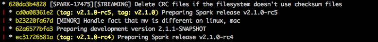
Spark’s release flow temporarily rewrites the POM to use Scala 2.10, releases that, then discards those changes, releases 2.11, and git tags that tree, leaving a git history like:
In ADAM, the POM changes are made into small _2.10- or _2.11-specific branches, each anchored by a git tag, which becomes the canonical SCM-pointer to each release:
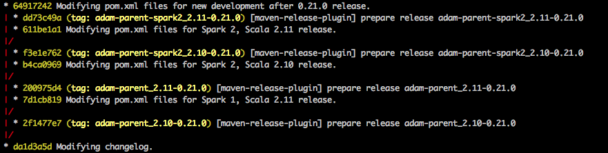
As you can see, a second, nested round of POM-regexing also happens (move_to_spark_2.sh) in order to publish for different Spark major-versions as well.
This is a bad state of affairs
Both of these workflows are distressing for several reasons:
- “Parsing” XML witih regexs is a famously bad/sloppy thing to do.
- The XML-“parsing” in question is not integrated with Maven at all.
- It resorts to
bash scripts, which fork to sed, despite its projects’ otherwise-deep buy-in to Maven’s project-management abstractions.
- Further pipelining/automation of release-processes are pushed to the lowest-common-denominator workflow-management tool, which is now
bash.
Spark is one of the biggest, most popular, and most active Apache projects; what hope do run-of-the-mill Scala projects have if this is the best release-workflow they can come up with?
Should people copy such a script into every Scala project they create?
It’s contagious
A little googling implies that Scala projects are, in fact, copying versions of this script around:
- here it is in Apache Zeppelin (2300+ GitHub stars),
- here in an Eclipse Foundation project called geomesa (200+ stars),
- here in Apache Bahir (80+ stars),
- here in Apache Flink (1800+ stars),
… the list seems to go on.
Presumably there is a better way…
Maven provides a deep set of abstractions for designing build-scapes:
- projects are configured entirely through Project Object Model (POM) XML files,
- a rich ecosystem of plugins supports XML-specification of ≈any workflow one may desire, and
- an opinionated set of default “phases”, “goals”, and “plugins” are added to projects by default.
I assumed this framework would allow me to express a trivial modification (s/_2\.10/_2\.11/g) to one of the basic POM attributes (<artifact/>; <version/> would also suffice), but I was wrong.
2000 Spoons
I attempted to make this work in Maven in myriad ways:
- Nest a property (e.g.
${scala.version.prefix}) in the <artifact/> tag, similarly to how most Scala-binary-version-dependent dependencies are expressed.
- Nest a property in the
<version/> tag, similarly to the above.
- Override either tag inside a
<profile/>.
- Define either tag in terms of an environment variable.
- Use
versions-maven-plugin to rewrite either tag.
- Upgrade/fork
versions-maven-plugin to be able to rewrite either tag.
- Write a Maven plugin from scratch for this purpose.
- Create a
<profile/> that invokes versions-maven-plugin followed by other build/release tasks, the latter ideally operating on a module whose artifact/version had been changed.
- Make the project’s root a POM-only parent-module (i.e.
<packaging>pom</packaging>), and then add JAR-packaged sub-modules for the _2.10 and _2.11 artifacts.
- (Mis)Use
maven-release-plugin and/or maven-deploy-plugin to override what artifact/version are released (according to some user-supplied configuration, e.g. a profile or property).
- Use classifiers, per a suggestion on this Spark dev list discussion.
All of these approaches failed.
Some discussion of specific failure-modes – and a sketch of an idea for actually accomplishing this with Maven – can be found in Appendix A, but suffice it to say that after being blocked in so many novel and frustrating ways from accomplishing something so simple, I began evaluating alternatives to Maven for my Scala-project-management needs.
SBT
SBT makes cross-publishing artifacts for different Scala versions trivial: you put a + in front of a task on the CLI, and it runs for all Scala-versions you’ve configured the project to build against.
For example:
sbt +publishSigned sonatypeRelease
builds JARs, POMs, source- and javadoc-JARs, and tests-JARs if desired (with corresponding sources- and javadoc-JARs), each for arbitrary Scala-binary-versions, and publishes the lot to Maven Central.
Beyond cross-publishing
While SBT clearly went out of its way to make cross-publishing trivial, the added power from configuring builds in Scala has also proved invaluable.
In short order I ported several dozen Scala projects to SBT, factoring out all repeated build-configuration to
hammerlab/sbt-parent along the way; my plan is now to use SBT for all Scala projects for the forseeable future, and recommend that others do the same.
Below I’ll drill in on specific pros and cons:
The Good
SBT gets several crucial things right:
“Key-value”-style configuration is succinct and sufficient in common cases
Consider this example from hammerlab/genomic-utils, setting a few project-level fields:
organization := "org.hammerlab.genomics"
name := "utils"
version := "1.2.0"
An equivalent pom.xml block would look like:
<groupId>org.hammerlab.genomics</groupId>
<artifactId>utils</artifactId>
<version>1.2.0</version>
which is comparably verbose.
In reality, the POM would have more boilerplate above and below this just supporting these values, and considerably more when expressing the remaining project configuration:
deps += libs.value('htsjdk)  // add a dependency, referenced by a name declared in the parent plugin
addSparkDeps                 // add dependencies on Spark, Kryo, and a test-scoped dependency on hammerlab/spark-tests
publishTestJar               // publish a "-tests" JAR, and attendant -sources and -javadoc JARs
The point is: Scala code can be made at least as lean for expressing simple attributes as any markup-language.
Where necessary, advanced language features can be deployed, and blocks factored out and reused
hammerlab/sbt-parent includes implementations of many repeated configuration blocks that have been factored out for concise re-use across projects.
Some examples in the wild:
Many more such conveniences can be found in the build.sbts of the modules in hammerlab/spark-genomics and by reading the hammerlab/sbt-parent implementation.
Plugin ecosystem parity with Maven
There seem to be functional plugins for all important tasks from the Maven ecosystem:
In some areas, SBT plugins exist that go beyond what I’ve observed to be possible in the Maven world, e.g. sbt-pack’s one-step creation of tarballs that can be make installed.
The Bad
In 2017, SBT is a lot more usable than at points in the past, but its learning curve remains steep. Some notes on classes of issues I hit:
Inscrutable and poorly-documented abstractions
SBT decomposes work into “tasks”, “settings” (special-cases of tasks), and “commands”; how/whether to compose/combine any of the three with any of the others, including themselves, is remarkably hard to understand.
However, even within this characterization there are some incorrect assumptions and caveats warranted, so a bit of feeling around in the dark is still inevitable when attempting any nontrivial pipelining.
A gem of SBT’s design is a lazily-eval’d computation-dependency-graph compiled statically from tasks’ references to other tasks/settings, using some macro-magic associated with a .value method on settings and keys.
As far as I can tell no one has tried to discuss how/why this works in a way that is remotely accessible to a non-SBT-committer.
This SO answer is the only discussion of it I’ve seen anywhere (incidentally, also linked to by sbt-coverage’s .gimme implementation above).
Ivy resolution
SBT uses a “latest wins” heuristic for resolving conflicting versions of dependencies: the newest version of a library found in the dependency tree will be used.
Maven, on the other hand, uses a “nearest wins” strategy: versions declared by dependencies closer to the root of the dependency tree are favored.
This discrepancy can lead to unexpected problems moving between Maven and SBT, or maintaining parallel builds; see this related configuration in Spark’s SBT build, and discussion on this example repo and in the SBT Gitter room.
The Gitter
In some low moments I was able to get help in the SBT Gitter room, particularly from @dwijnand (thanks! 😀).
Among other things, he recommended this excellent blog post as a starting point for understanding SBT’s design/API, which was very helpful.
Conclusion
Doing away with the daily indignities of trying to serialize simple build-logic into Maven’s uncooperative POM framework has been a boon to my ability to create, release, and maintain Scala projects, and I hope that my travelogue here will help others in similar situations.
Realizing that I wanted/needed as much from language/tooling when configuring my builds as I do when writing the code that I later seek to build was an important epiphany, and has led to further revelations about missing functionality in the larger JVM-ecosystem-project-management universe, that I hope to touch on in subsequent posts.
Feel free to drop by any of the hammerlab-org repos linked here, or our public slack channel, to discuss further!
Appendix
A: Trying and Failing to Scala-cross-publish with Maven
The following are notes on a couple of attempts to set up a Maven-based workflow for cross-publishing differing Scala-binary-versioned artifacts:
Rewriting POMs
Several things I explored involved rewriting POMs, like a change-scala-version.sh does, but perhaps with a real XML parser or in a way that is somehow better-integrated with other Maven workflows.
At the end of the day I found this approach to be suboptimal at a high level: Maven only picks up POM-changes when a new invocation is run, and this feels like a basic breach of the dependency-/worfklow-management contract.
In any case, here are some such attempts that were nevertheless unworkable:
This plugin is in wide use for doing things sort of like what is required for cross-publishing Scala-binary-versioned artifacts, but on investigation I found it to not facilitate much improvement over the status quo.
Its Maven phase parses the POM XML, rewrites the appropriate <version/> tag(s) (with… fake XPaths?), and then writes the POM back out, taking care to preserve whitespace and any POM-formatting idiosyncracies. Subsequent mvn-CLI invocations then pick up the values in the rewritten POM.
That sounds like an improvement, but would basically require two actions to run:
- rewriting
<artifact/>, using a new function similar to ones in POMHelper
- updating the
${scala.binary.version} property typically used for qualifying dependencies.
Digging in, I found that the plugin adds some overhead to this (values it splices in must be versions of dependencies that it is aware of), and the end-result would still be an unsatisfying rewrite-the-POM-then-run-again state of affairs, so I gave up on this approach.
Like versions-maven-plugin, this plugin is used for similar POM manipulations to those we might desire, e.g. rewriting a bunch of <version/> tags using an XML parser.
Also like versions-maven-plugin, unfortunately, its operations are only picked up by subsequent Maven invocations, which breaks the .
BYOPlugin
I prototyped a custom Maven plugin for doing POM rewrites similar to those discussed above, but was stymied; for one, I wanted to write my plugin in Scala, but this generated the kind of errors (and corresponding empty SERPs) that made me feel that no one had ever attempted as much before, and that it wasn’t likely to be workable.
As also mentioned above, I was also pursuing the “POM-rewriting” approach, not appreciating that what I really wanted was an altogether different model, discussed below.
Coloring inside the lines
A couple of approaches sought to use existing Maven-plugin XML APIs to do what I want; they also failed!
I thought I might solve cross-publishing by having a POM for each Scala-binary-version I wanted to publish for, and a parent POM that wrapped 2.10 and 2.11 submodules.
Of course, almost everything would be reused in both modules’ POMs, so you’d want most things (like <dependencies/>) specified in the parent.
However, I ran aground: some ${scala.version.prefix} had to be set in the parent-POM that was published, and the child/implementation modules inevitably inherited whatever was set there: I was back to needing to cross-publish the parent POM, or repeat all dependencies in each child POM.
In discussion of an early draft of this post, @vanzin pointed me to this attempt at solving this problem, which is used in production by cloudera/livy.
At the time of this writing, my understanding is that it faces the same problem described above, per vanzin/multi-scala#1.
Maven <classifier/>s
AFAICT, classifiers can’t be made to solve this, because Scala 2.10 and 2.11 releases require not just JARs with different names and binary contents, but different dependencies as specified in the POM; this seems to require separate POMs, and therefore separate (group,artifact,version) tuples.
“If I knew then what I know now”
I think that one could write a Maven plugin that, instead of rewriting POMs and requiring a Maven reboot, used APIs like MavenProject.setArtifactId to modify internal Maven state that would govern how all of its usual phases operated.
You could then have a <profile/> – ideally defined in a parent-POM that Scala projects inherited, to minimize boilerplate – that activated a custom plugin phase that changed the <artifact/> and <${scala.binary.version}/> before proceeding through all requested phases, without messing with transient POM changes or Maven reboots.
B: Pants
As mentioned at the start of the post, I also experimented with porting some repos to Pants.
Pants’ design has some desirable properties over all other tools that I’m aware of:
- explicit tracking and caching of workflow-nodes’ inputs and outputs,
- support for caching outputs globally (e.g. across an organization),
- automatic analysis/pruning of dependencies,
- etc.
However, the open-source community / support-base around it is significantly smaller than that of Maven and SBT, and it felt like I’d have to write some plugins myself, in Python, which proved to be a dealbreaker given the option to write build logic in Scala instead.
I hope some of the great features of Pants will become more accessible soon, or that other tools will incorporate them!
30 Nov 2016
| by
Jacki Novik
and
Tavi Nathanson
Cohorts is a Python library for managing, analyzing and plotting clinical and genetic data from patient cohorts. It was spun out of our work analyzing data from clinical trials of checkpoint blockade in melanoma, lung, and bladder cancer. The sponsors of these trials typically collect a wide range of data for each patient in order to discover and evaluate potential biomarkers for association with benefit from therapy. While some aspects of Cohorts are specific to that context (e.g. the integration with neoantigen prediction), other components are more generally usable.
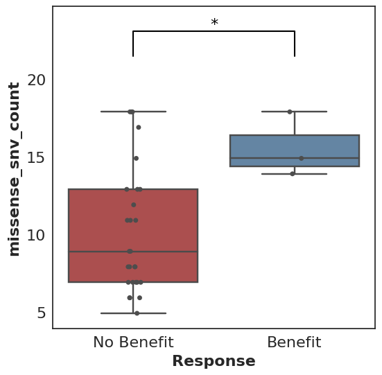
A prototypical use case for Cohorts is a Mann-Whitney comparison and associated box plot of the number of missense SNV mutations found in patients who did benefit from therapy (where benefit is defined by the user, e.g. progression-free survival greater than 6 months) versus those who did not benefit.
In its simplest form, this looks like:
cohort.plot_benefit(on=missense_snv_count)
But where does this cohort come from, what is this missense_snv_count, and what else can we plot? Let’s explore how Cohorts works!
Note: all code in this post is available in a Jupyter notebook.
Creating a Cohort
A cohort must be populated before analysis and plotting can proceed. Within Cohorts, each Cohort consists of a set of Patients, each of whom may have tumor and normal Samples.
Samples hold paths to associated BAM files as well as Cufflinks or kallisto output. Patients contain key clinical variables (clinical benefit status, overall survival, progression-free survival, deceased status, progression status), tumor and normal Samples, paths to tumor-normal VCFs, HLA alleles, as well as any additional relevant data. Cohorts contain all Patients as well as a variety of cohort-level settings.
Patients do not need to contain Samples, and they won’t when used for purely clinical data analyses. If you have data that isn’t easily modeled as described, but would like to make use of Cohorts, please file an issue on GitHub!
Analyzing a Cohort
The analysis and plotting functions of Cohorts generally rely on Pandas DataFrames. The simplest way to begin analysis is via direct access to the DataFrames that Cohorts produces. For example:
df = cohort.as_dataframe()
To go further, Cohorts will enhance user-provided data by calling out to external libraries like Topiary, Varcode and Isovar. These results are then exposed as potential biomarker datapoints for analysis.
For example, the function missense_snv_count, which requires paths to SNV VCF(s) to be specified in the Patients, utilizes Varcode to filter those mutations to those that are missense. neoantigen_count uses Topiary to compute predicted neoantigens from those SNVs.
These functions can be plugged into Cohorts:
# Return a DataFrame with "neoantigen_count" as a column,
# in addition to user-specified patient data.
df = cohort.as_dataframe(on=neoantigen_count)

# Return a DataFrame with "Neoantigen Count" and
# "Missense SNV Count" as additional columns.
df = cohort.as_dataframe(on={"Neoantigen Count": neoantigen_count, "Missense SNV Count": missense_snv_count})
While a number of these data-enhancing functions are available out of the box, users can always write their own custom functions to support their analyses of interest.
Below is a simple custom function example:
def smoker_or_senior(row):
    return row["smoker"] == True or row["age"] >= 65
This can be used just like the functions above:
df = cohort.as_dataframe(on=smoker_or_senior)
Plotting
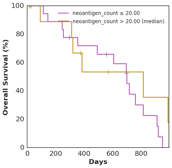
In addition to plot_benefit, Cohorts comes with various analysis and plotting functions. To name a few: plot_survival, plot_correlation, coxph, and bootstrap_auc. plot_survival uses Lifelines to plot two survival curves split by a specified variable. The following code generates a survival curve for patients with more neoantigens than the median and a survival curve for patients with fewer, based on Topiary’s neoantigen prediction:
cohort.plot_survival(on=neoantigen_count)
Analyses and plots based only on data supplied directly to the Patient, as opposed to computed features using data-enhancing functions, are also fair game:
# note: resultant image not shown here
cohort.plot_survival(on="smoker")
For binary features, Fisher’s exact test is used along with an associated bar plot:
cohort.plot_benefit(on="smoker")
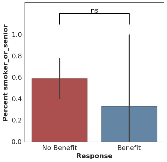
All calls to plot_benefit result in a p-value significance indicator at the top of the plot, thresholded by 0.05 by default (* for significant and ns for not significant).
Results from other data locations can be loaded into an analysis using join_with:
# note: resultant images not shown here
cohort.plot_benefit(on="PD-L1 Expression", join_with="pdl1")
cohort.plot_correlation(on={"Missense SNV Count": missense_snv_count,
                            "PD-L1 Expression": "PD-L1 Expression"},
                        join_with="pdl1")
The above uses a DataFrameLoader, which is defined when a Cohort is created. It associates "pdl1" with a given DataFrame and specifies how to join that DataFrame with the Cohort. We typically load results from IHC analysis, tumor clonality estimates, mutational signature deconvolution, and TCR-Seq in this way. While extra data sources can also be added to the Cohort data itself to avoid joining (see Patient.additional_data), keeping certain data sources separate is helpful when a data source has a one-to-many relationship with the Cohort or is slow to load.
Consistency and Reproducibility
Many of the features in Cohorts have a goal of promoting consistency and reproducibility across various analyses. Examples include:
Variant Filtering
A user can define custom variant filtering functions, and filter variants accordingly. For example:
# Filter variants to those with at least 3 reads in the tumor sample.
def tumor_read_filter(filterable_variant):
    somatic_stats = variant_stats_from_variant(
        filterable_variant.variant,
        filterable_variant.variant_metadata)
    return somatic_stats.tumor_stats.depth >= 3

# Use a default filter function for the Cohort.
# note: resultant images not shown here
cohort.filter_fn = tumor_read_filter
cohort.plot_survival(on=missense_snv_count)

# ...or specify a filter function ad-hoc.
cohort.plot_survival(on=missense_snv_count,
                     filter_fn=alternative_filter)
Data Caching and Provenance
Cohorts caches many results, such as variant effects and predicted neoantigens, to mitigate the computational overhead frequently involved. A file-based approach enables easy sharing and manipulation of cached objects.
Cohorts also keeps track of the context in which the cache was generated by tracking the versions of software used to generate the cache. This context, as well as a hash of the base (unenhanced) data, is available for printing and optional version checking.
Other Resources
Ready to take Cohorts for a spin? The following notebooks should help you get started:
We’d love to hear from you if you have any feedback, suggestions, or bug reports!
01 Nov 2016
| by
Leo Rozenberg
The MHC gene family is well known for its polymorphism.
The IPD-IMGT/HLA database provides the official reference
sequences for the alleles found in this region.
In addition, the Anthony Nolan HLA informatics group provides a
reference alignment of these alleles.
Here is a pared clip (we insert ellipses to skip lines) of the output for the
genetic DNA of HLA-A:
This format textually encodes differences between the reference sequence (the
first one, A*01:01:01:01) and the other, alternate, allele sequences, along
the file columns.
Using special characters, the reader can tell if the alternate nucleotide
is unknown (‘*’), the same (‘-‘), different (‘A’, ‘C’ …etc), or a gap (‘.’)
to the known reference nucleotide in the same column.
While this format has its place, it isn’t useful for quickly
visualizing the diversity of this region. We’ve created a small utility
to marginally improve visualizing these alignments.
mhc2gpdf
Our first intuition for this task was to compress the redundant
sequence information.
Grouping shared sequence segments as nodes
led to us thinking about the entire alignment as a graph,
and from this starting premise some properties followed naturally:
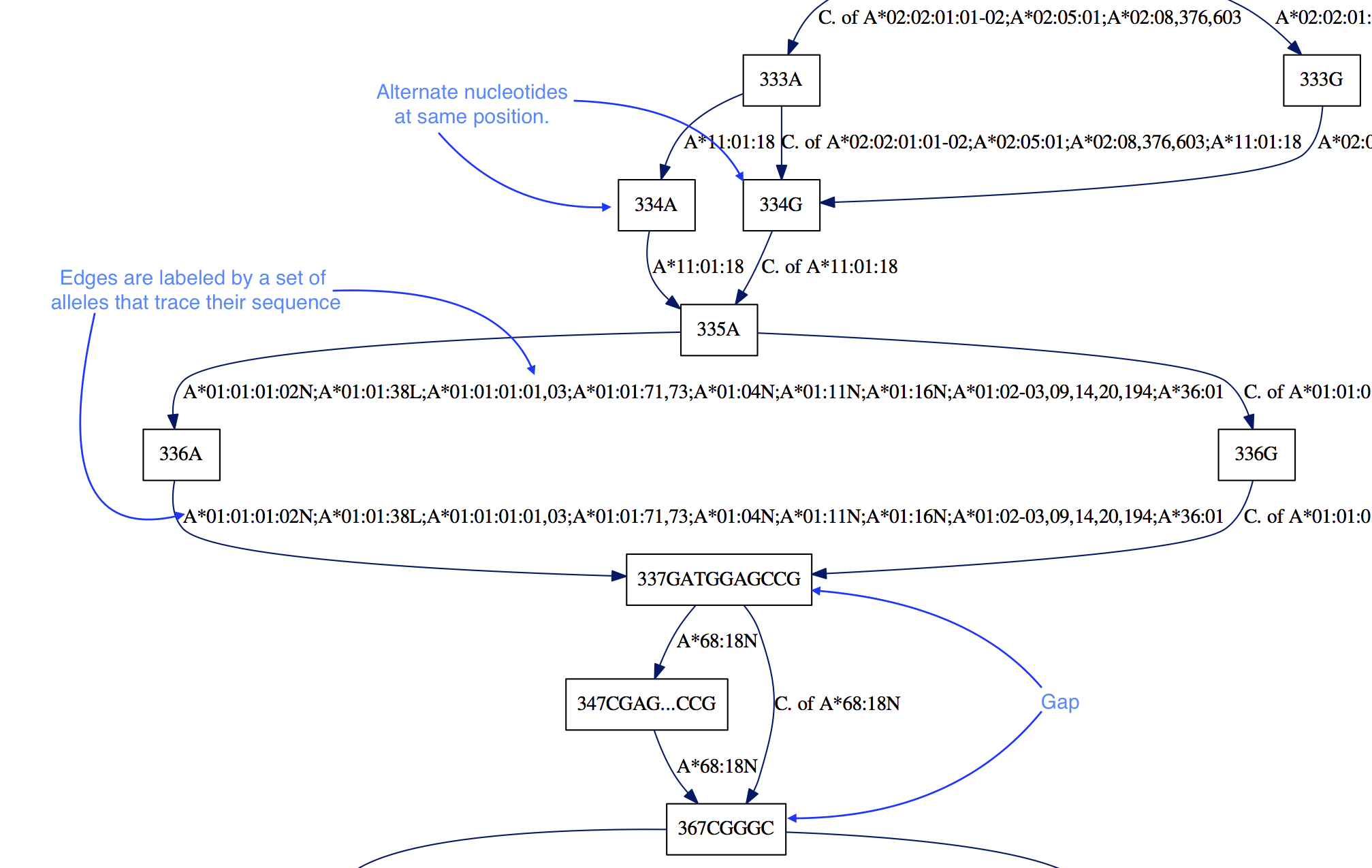
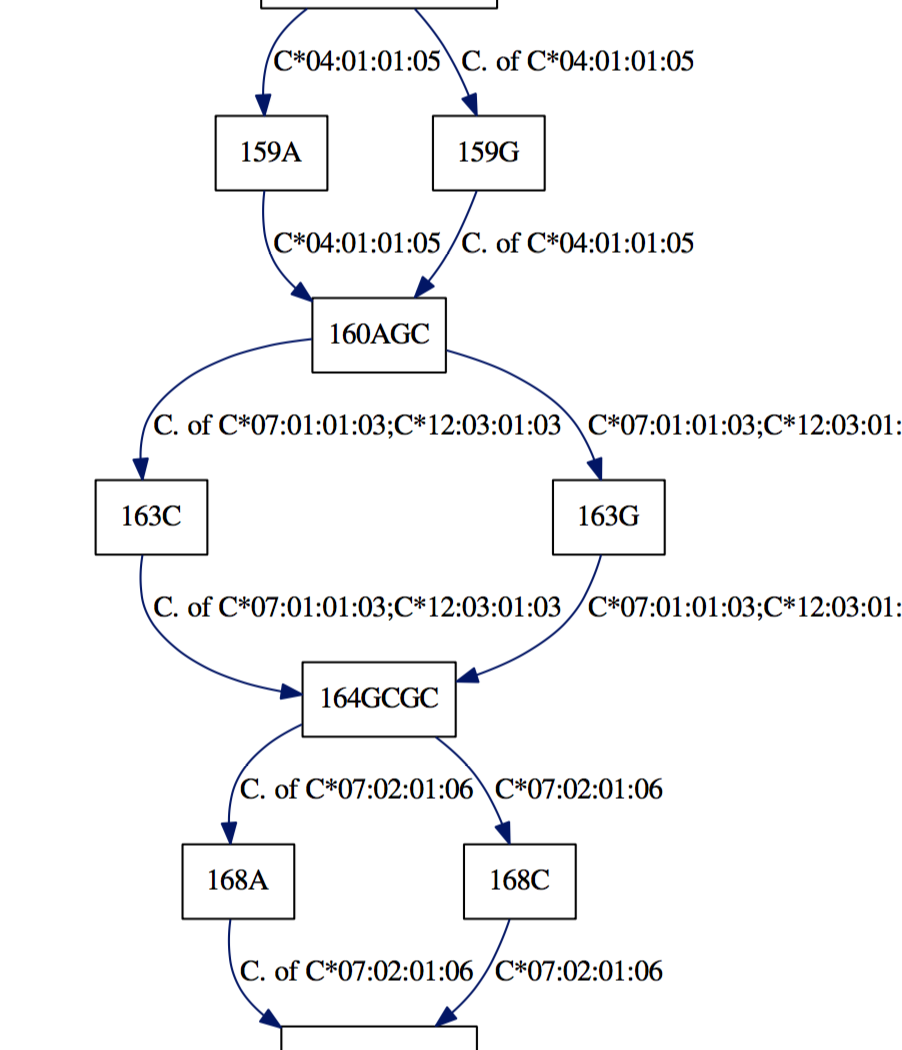
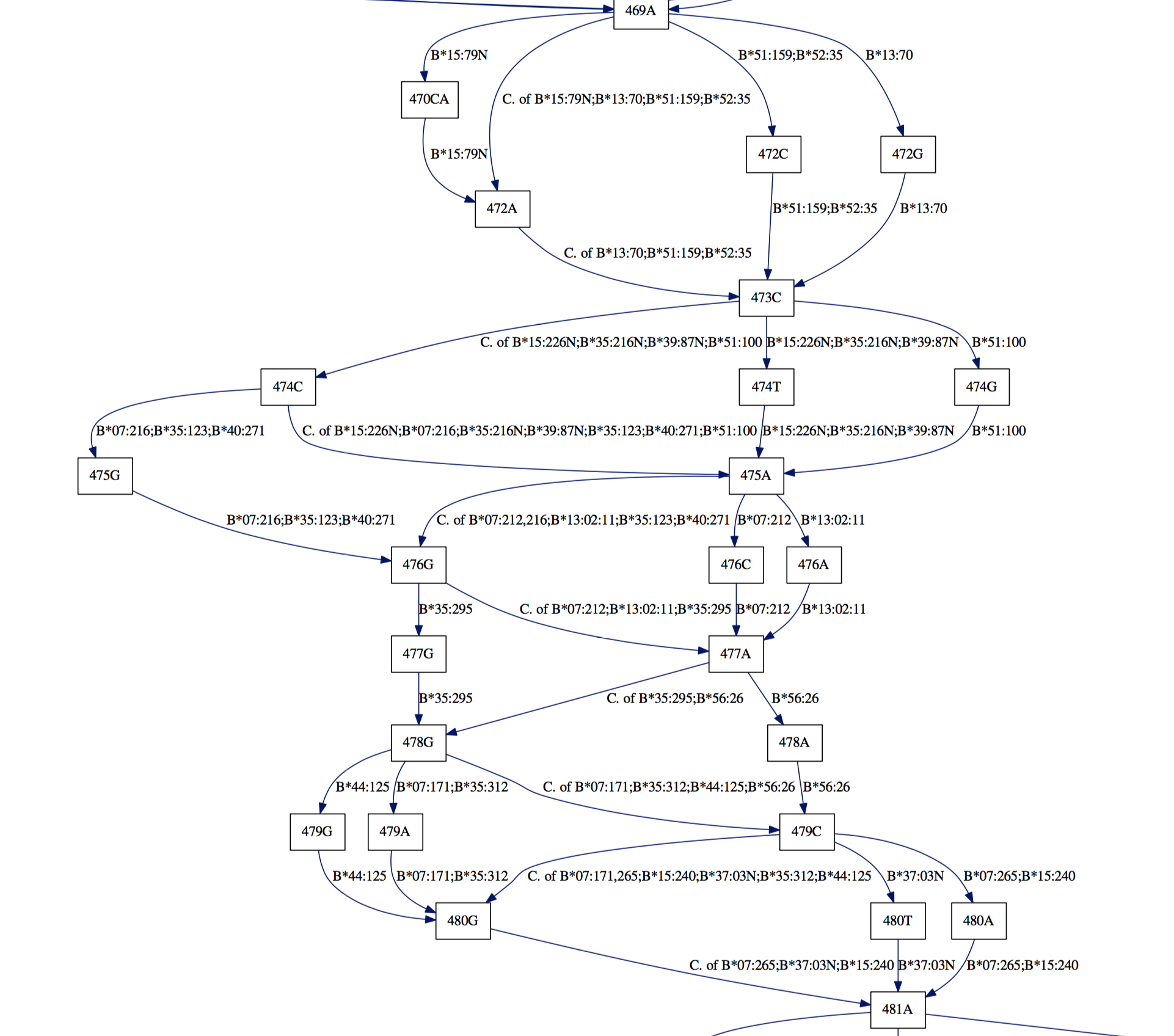
- Alleles are represented by edges, such that one can trace
the sequence of the allele by following edges.
- Alignment information is preserved by adding a numerical label of
alignment position. Different nucleotides at the same position are
represented by different nodes: “336A” vs “336G”.
- Gaps are encoded by the edges that point to nodes with a position
farther than the position at the “end” of a node (the start label plus the
length of the node sequence). In the example above, the “337GATGGAGCCG”
node ends its position at 347 since
len(GATGGAGCCG) = 10.
Therefore there is a 20 nucleotide gap, in all of the alleles except
“A*68:18N”, as indicated by the edge to “367CGGGC”.
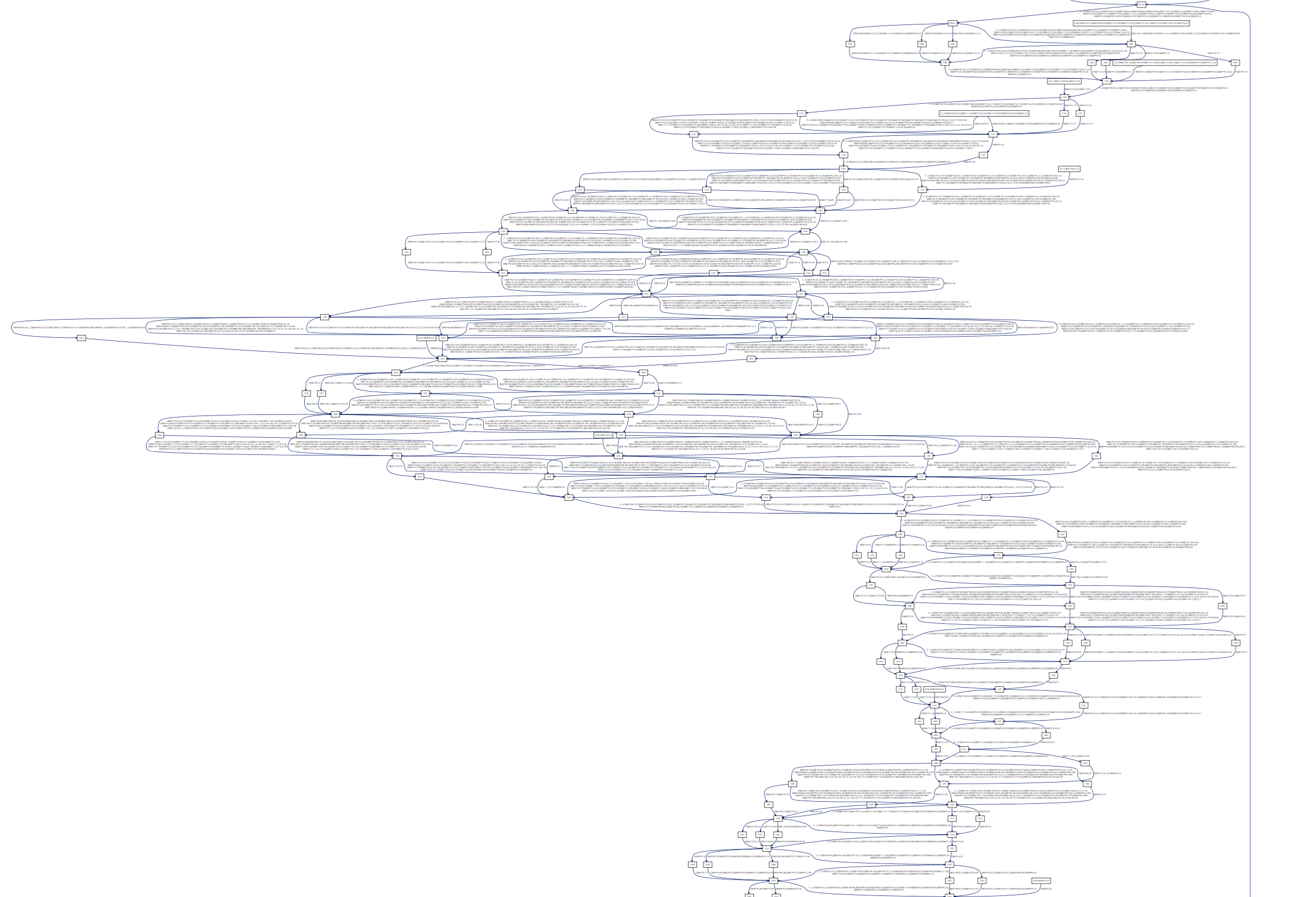
Underneath the hood, mhc2gpdf first parses the alignment file;
then constructs the desired graph representation by creating
the desired nodes and edges;
finally, it writes a dot file and calls Graphviz to
render the dot file to PDF.
Samples
With these pdfs we can quickly determine allelic differences:
Appreciate the dense polymorphism of these genes:
And see long gaps in the Class II DRB nucleic sequences:
We’ve used our tool on the latest IMGT release (2016-10-19) and
provide the dot and rendered pdfs: happy browsing!
Reading the graph
We’ve made some stylistic choices to make the graph easier to understand:
- We run-length encode the leaf nodes of the tree that represents the
allele edges: instead of “A*01:01:02,A*01:01:04,A*01:01:05…A*01:01:37”,
we’ll write “A*01:01:02,04-37”.
- If an edge represents more than half of the allele set, we’ll describe
its complement and prefix the string with a “C. of”, short for
“Complement of”.
- We add “Start” nodes, prefixed with an “S” to indicate where the alignment
has sequence data for each allele. These are similarly encoded as the
edges.
- We add “End” nodes for the same reason. These just have the final position.
- We add “Boundary” nodes, which are represented by “|” in the alignment
file for exome boundaries.
Feedback
We hope that the genetics community finds this tool useful and we look forward
to your feedback on GitHub.
23 Feb 2016
Gene Set Enrichment Analysis (GSEA) is a well-known and widely-used method in Computational Biology and Bioinformatics. GSEA uses a sorted list of genes (obtained by comparing gene expression levels between groups of patients) and a database of gene sets as input, and it checks whether members of a particular gene set have a non-random ordering, biasing them towards the top or the bottom of the list (i.e. enrichment). We leave the details of the method out of this blog post, but the original paper describing GSEA is a good starting point for newcomers.
Gene sets often represent biologically meaningful groupings: for example, all genes that are active during controlled cell death. It is common to see these gene sets being referred as pathways and it is for this reason that GSEA is also known as pathway analysis. This name, unfortunately, leads to the following misconceptions regarding the whole approach: 1) Pathways are well-defined gene sets and they do not change; 2) There is no room for customization of the database of gene sets used in the enrichment analysis.
First, there is no clear consensus over the contents of a pathway across many of the databases, let alone the researchers, and therefore our knowledge on the list of genes that are members of a particular pathway is constantly evolving. This means that our database of gene sets should evolve with our knowledge, but in reality, it is far behind our current knowledge due to the slow nature of the literature-based curation process.
Second, the enrichment analysis does not necessarily depend on default data sets and is flexible enough to work against custom gene set definitions when needed. As long as a researcher is confident that the gene sets used in the enrichment analysis reflect our current knowledge regarding biological processes and they are uniformly curated, there is no need to worry about using custom data sets as gene sets.
New Cancer Immunology Collections in GSEA
As part of one of our research projects focusing on immunotherapy in cancer, we needed to run GSEA on a gene expression data set to explore enrichments in patients with different outcomes (phenotypes). Our sample size was on the order of tens, which meant that we had low statistical power for the analysis. To account for this, we decided to stick to only one of the curated gene sets; but this collection was lacking gene sets that were highly interesting to us. Specifically we were interested in including tumor-associated antigens recognized by CD4+/8+ T-cells and gene signatures associated with immune cell infiltration to the tissue.
Our solution to this was to collect curated gene lists from relevant resources that are not part of the MSigDB, extract the official gene symbols and include them in our analysis as additional gene set collections. For the former, we used the up-to-date list of tumor-associated antigens from Cancer Immunity’s Peptide Database; and for the latter, we used gene sets inferred by Senbabaoglu et al that builds on the work of Bindea et al and infers gene expression signatures associated with immune cell filtration in kidney cancer:
Creating GSEA-compatible gene set collections
You will see from the examples above that the default Gene Matrix Transposed (GMT) file format features a separate gene set on each row, two metadata columns for each gene set followed by an arbitrary number of gene identifiers that belong to the corresponding gene set. The file format, therefore, is an extension of tab-separated values (TSV), meaning that almost any text editor or other third party software that can handle TSV format can be used to curate these files.
One way to tackle this problem is to generate these files programmatically and often researchers are interested in adding new gene sets to the analysis based on lists of genes published as supplemental material to papers. A practical solution that works nicely for us is to import such gene sets into Google Spreadsheets (for collaborative editing, taking care to ensure that gene names aren’t converted to dates) and then reduce them to GMT files to be used in the analysis. You can find a Python-based solution to this common task in this notebook as an example that converts gene lists extracted from the papers we mentioned above and turns them into individual GMT files.
Some words of caution about custom gene sets
Although adding one or more custom gene sets into the analysis is pretty straightforward, it still requires careful planning and some basic bioinformatics skills. It is, for example, really important to be consistent with the use of common identifiers across default and custom collections. Not all gene sets are curated with gene identifiers that are consistent across databases; therefore, gene identification mapping from one provider to another often becomes essential. Note that problems in such mappings can easily cause over- or under-representation of gene sets due to cross identification mismatches.
Furthermore, once these custom gene sets start accumulating, it becomes important to check the degree of overlap across multiple gene set collections to prevent redundant enrichment tests. Although this is an imperfect science, one way to check this would be to compare all pairs of gene sets across two GMT files and calculate an asymmetric score that represents to what extent the first collection is represented within the second collection.
Another thing to consider when using custom gene sets in the analysis is to run the analysis on the combined collection of gene sets (including both the default and the custom ones) and not individually to properly account for false discovery rate. With that, it often does not make sense to restrict the analysis to only the custom gene set, but it is good practice to combine it with another collection as a good background for the enrichment tests.
Final words
It is crucial for the community to share such custom gene sets and explain the rationale behind them for encouraging others to build on such efforts. We wanted to share our experience and solutions that worked for us so that not everybody has to reinvent the wheel.
09 Dec 2015
We’ve spent the past year building pileup.js, an interactive JavaScript genome browser. We’ve used Facebook’s Flow system throughout the development process to bring the benefits of static type analysis to our code. This post describes our experiences and provides some advice for getting the most benefit out of Flow.
What are the benefits of using Flow?
The most often-cited rationales for type systems are that they:
- Catch errors early
- Improve readability of code
- Facilitate tooling
- Improve runtime performance
In the case of Flow, runtime performance is not in play. The other factors are the main motivators.
For catching errors early, Flow winds up being a great way to avoid round-trips through the “save and reload in the browser” cycle. If you use Flow throughout your code, you’ll see far fewer Syntax Errors or undefined is not a function messages pop up in your JavaScript console. Similarly, it’s a huge help in refactoring. If you rename a module or function, Flow will immediately find all the references to the old name.
That being said, this aspect of Flow has proven to be mostly a time saver, rather than an effective way to find bugs. Most egregious bugs would have been caught by a unit test or manual testing before they were ever committed to source control. The type system just lets us find them more quickly.
The primary long-term reason to use Flow (or TypeScript) is for the improved readability of code. Far too often in JavaScript (or Python), you’ll run into a function like this:
function updateUI(data) {
  ...
}
It was surely obvious to whomever wrote the function (perhaps you, six months ago!) what data was. You’d sure like to update the UI. But what exactly do you pass to this function? For simple code, you may be able to infer the parameter type by inspection. But for complex functions which call out to other functions in other modules, this quickly becomes difficult. Type annotations and type inference can both immediately tell you what’s expected.
For large codebases, this winds up being a huge aid. Complex UIs often use large, nested objects to represent their state. This is very common with React Components, for example. With type annotations, it’s clear what type of object each component expects. And, if you’re still confused, Flow will let you know. What’s more, unlike types which are documented in comments, you can be confident that type annotations are up-to-date and correct. If they weren’t, Flow would have complained.
Why use Flow instead of TypeScript?
An aside: why did we use Flow instead of TypeScript? When we started work on pileup.js, TypeScript had poor support for both Node-style require statements and for React.js and its JSX syntax. These issues are both less relevant now: both Flow and TS support ES6 import statements, which is what all projects should be using going forward. TypeScript 1.6 added support for JSX, so that’s less relevant too.
Both Flow and TypeScript are good choices for a new project. Flow is a more sophisticated type system, with better support for patterns like type unions and nullable types. TypeScript is more established and has better support, e.g. more editor plugins and third-party type definitions.
Practical experiences / gotchas
Editor integration
While you can run flow check and flow status from the command line and as part of your continuous integration, you’ll be missing out on many of its benefits if this is all you do. Flow works best when it integrates with your editor. With the vim-flow plugin, for example, Flow will show any new errors inside of vim whenever you save a JS file. This is fast (or should be – see below!) and helps you catch errors without the context switch of going to your web browser.
Flow is a server
Flow is intended to be run as a background server. When you run flow status, it starts up the server, reads and analyzes all your code and then waits for files to change. When you run flow status again, you’re just asking the server for the latest errors. Incremental changes are fast, but the server startup is slow. flow check runs a full check and is always slow. So use flow status, except in contexts which are not latency-sensitive, e.g. your continuous integration build.
Sometimes you’ll make a change that forces the Flow server to restart. These include changes to your .flowconfig file or changes to a type declaration (lib) file. There’s no way around this. You’ll just have to wait 20-30 seconds to get type errors again.
Flow reads your entire node_modules directory
Incremental compiles should take under a second. You can check this time for your project by running:
echo '' >> some/js/file.js; time flow status
If this time gets too large (e.g. more than a second), it might be because Flow is wasting time reading everything under node_modules. You can check how many files Flow is tracking by running this sequence:
flow check --verbose 2> /tmp/flow-all.txt
grep -o '/node_modules.*' /tmp/flow-all.txt | perl -pe 's/:.*//; s/[\\]?".*//; s/ .*//' | sort | uniq | wc -l
If this is significantly larger than the number of JS files in your project, then Flow is wasting time. You should add as much of node_modules as you can to the [ignore] section of your .flowconfig. See this issue for details.
Creeping any types
One of the pitches for Flow is that it performs type inference on your JavaScript. You don’t even have to provide type annotations, Flow will figure out your code! For a few reasons, however, this does not work in practice. First, Flow requires that you explicitly annotate all functions and classes which are exported from modules (this is for performance reasons). Secondly, there are many ways that any types can creep into Flow code:
- Third-party libraries If you import a third-party module (e.g. underscore), then the type of the entire module will be
any. This means that any data that passes through functions in that module will come out with an any type. The solution to this is to use a type declaration file. While there is some movement towards providing a central registry of Flow type definitions, it’s nowhere near as mature as TypeScript’s DefinitelyTyped.
-
Props and State If you use React, you need to explicitly specify types for your props and state. Otherwise, they default to any. You can get slightly better behavior by using propTypes, which Flow understands. But the best way is to explicitly define types for props and state using an ES6 class:
type Props = {
  name: string;  // note: not null!
  address: string;
};

class AddressBookEntry extends
    React.Component<void /* DefaultProps */,
                    Props,
                    void /* state -- none in this component */> {
  ...
}
This will check types for props, state and setState within your component. It will also check the props on AddressBookEntry when you create one using JSX syntax elsewhere in your code (i.e. <AddressBookEntry name="Dan" /> would be an error because address is missing). If you define props and state members, you will get the former but not the latter check.
- Missing @flow annotations If you forget to put
@flow at the top of your source file, Flow will ignore it by making its type any. We added a lint check to ensure that all our JS files had this annotation.
You can run flow coverage path/to/file.js to see the fraction of expressions in a file whose type is any. You should try to keep this as low as possible. The :FlowType vim command shows you what Flow thinks the type of the expression under your cursor is. This can also help to find gaps in what Flow will catch.
Surprising non-errors
JavaScript is a very permissive language. Flow models some elements of this permissiveness but disallows others. For example, '1' + 1 evaluates to '11'. Flow complains about this because it’s likely to be a mistake (and at the very least indicates unclear thinking).
JavaScript also allows you to pass any number of arguments to functions. For example, Math.pow(2, 4, 6, 8) == 16. Arguments after the second are simply ignored. This is also likely to be a mistake, but Flow is OK with passing too many arguments. Other examples include functions are objects.
We often find ourselves wondering “would Flow catch this?” It’s a good habit to introduce errors and typos to double-check that Flow is understanding your code.
Misattributed / cryptic errors
Many students have a sinking realization during their Compilers classes that, while parsing a correctly-formed program is fun and easy, 95% of the challenge in writing a good parser is the tedious process of catching errors, determining where they are, and recovering from them.
Something similar seems to be at play with Flow. If Flow reports that there are no errors, then (modulo any types and non-errors, see above) you can be confident that there are none. If it reports a problem, then there probably is one. But the error message may or may not point you in the right direction. There are many open issues around error messages.
For example, we’ve learned from experience that intersection types can be a source of cryptic errors. For example:
var el = document.createElement('canvas');
var ctx = el.getContext('2d');
ctx.fillRect(0, 0, 200, 100);
This produces an odd-looking error:
2:     var ctx = el.getContext('2d');
                 ^^^^^^^^^^^^^^^^^^^ call of method `getContext`. Function cannot be called on
2:     var ctx = el.getContext('2d');
                 ^^^^^^^^^^^^^^^^^^^ HTMLCanvasElement
getContext is most certainly a method on HTMLCanvasElement. The real issue is on the third line, not the second. getContext is allowed to return null, which does not have a fillRect method. This error bubbles up to the point where these two cases diverge, resulting in the cryptic message. The solution is to add an if (ctx) { ... } check around the drawing code.
This example illustrates both the strengths and weaknesses of Flow. It’s impressive that Flow can track the way that functions return different types based on parameter values, e.g. HTMLCanvasElement from document.createElement('canvas'). This eliminates a common source of typecasts in other type systems. It also illustrates a case where null-checking is not helpful. In practice, getContext('2d') will not return null.
Conclusions
Flow is a powerful tool for performing static type analysis on JavaScript
codebases, bringing their maintainers many of the benefits that this yields.
Flow is not without its quirks, though, some of which we’ve documented here.
Understanding these will help you get the most benefit out of Flow.
Flow is developing rapidly, with dozens of commits being merged
every week. This is one of the very best things about it. In the year that
we’ve been using it, many new features have been added and many fundamental
issues have been resolved. It’s likely (we hope!) that some of the gotchas in
this post will no longer be gotchas by the time you read it.