26 Jun 2017
| by
Jacki Novik
Survival analysis is an important and useful tool in biostatistics. It is commonly used in the analysis of clinical trial data, where the time to a clinical event is a primary endpoint. This endpoint may or may not be observed for all patients during the study’s follow-up period.
At the core of survival analysis is the relationship between hazard and survival. The observed time to event \( t \) or Survival is often modeled as the result of an accumulation of event-related risks or hazards at each moment up to that time \( t \). Factors that modify the time to event do so by reducing or increasing the instantaneous risk of the event in a particular time period.
The basic survival model posits quite an elegant relationship between covariates and the dependent variable. In addition, there are several analytical problems that survival analysis attempts to address, which may not be obvious at first glance.
Among these, I would highlight the following:
-
Time-dependent risk sets: At each time t, only a subset of the study population is at risk for the event of interest. For example, if the primary endpoint is death, we should only expect to observe this event among patients who are alive at a time t. The calculation of an event rate at any point during follow-up should consider only those patients eligible for the event.
-
Censoring of events: Typically there is a subset of patients for whom the primary endpoint was not observed. For these patients, the endpoint is said to be censored. For these patients who did not experience an event, all we know is the last time that patient was observed event-free.
One of the most common approaches to survival analysis is the Cox Proportional Hazards (Cox PH) model, which was first proposed by David Cox in a 1972 publication. However, survival modeling and particularly Bayesian survival modeling continues to be an area of active research. There are several more recent developments which we are interested in applying to our research, which aims to discover biomarkers for response to immune checkpoint blockade in the context of cancer.
In particular:
We developed SurvivalStan in order to support our own work implementing many of the methods described above in Stan and applying them to analysis of cohorts treated with immunotherapy.
In the following introduction, we will give a brief introduction to survival analysis and the standard set of assumptions made by this approach. We will then illustrate applied examples from our own research, including:
- A piecewise exponential model
- A varying-coefficient analysis
- Estimation of time-dependent effects
Many of these examples (and more) are included in the documentation for SurvivalStan, available online. We welcome feedback on this package in our github repo.
Motivations
Many of the methods described above have been implemented in user-friendly packages in R, so one may argue that we don’t need yet another package for survival analysis. However, these packages are in some ways too robust for our use case.
In our research we need to be able to iterate on the model fairly quickly. Also, given the considerable complexity of the models and our interest in exploring the full posteriors of said models, we want to use NUTS and Stan to fit our models. Having a number of modeling approaches fit using the same inference algorithm allows one to do better model comparison.
We also want it to be easy to apply the models to a dataset for publication or discussion. In support of this goal, we have included a set of functions for pre-processing data and for summarizing parameter estimates from the model.
We finally value reliability of the models and so have made efforts to check the models against simulated data routinely, as part of our travis tests. There is (always!) more work to be done in this area, so use your judgement when applying these models, but the main pieces of this are in place.
It is our hope that other researchers will find the package useful, and that some may even contribute additional models according to their application.
Leveraging the power of Stan
We have therefore designed SurvivalStan to:
- Support common tasks in Survival modeling, such as preparing data for analysis or summarizing posterior inference
- Provide Stan code for standard models, where each model is a single file that can be edited for specific applications
- Allow the user to supply a custom Stan model, to enable a greater range of options than those supplied by default
- Provide a robust testing environment to encourage routine checking of models against simulated data
This paradigm breaks with that utilized by some of the excellent packages which expose Stan models for wider consumption such as rstanarm, which (a) pre-compile models on package install, and (b) utilize complicated logic within the Stan code for computational efficiency and to support a wide variety of user options. These design decisions make sense for that use case, but not for ours.
By comparison, the Stan code included in SurvivalStan is focused on a particular model and so is only as complex as that model demands. Flexibility is instead supported by including more Stan files (roughly one per baseline hazard type) and by supporting direct editing of any of these Stan files. The expectation is that users will be fairly sophisticated – that is, familiar with the Bayesian modeling process, how to evaluate convergence, and the importance of model checking.
What SurvivalStan instead provides are utilities for data preparation for analysis, calling out to pystan to fit the model, and summarizing results of the fitted models in a manner appropriate for survival analysis.
Below we will work through some examples illustrating the variety of models one can fit using SurvivalStan. Reproducible code is available in the example-notebooks included in the package repo.
A Very Brief Introduction to Survival Modeling
Let’s start with a brief introduction to establish key terms.
Recall that, in the context of survival modeling, we have two functions :
-
A function for Survival (\( S \)), i.e. the probability of surviving to time \( t \):
where the true Survival time is Y.
-
A function for the instantaneous hazard \( \lambda \), i.e. the probability of a failure event occurring in the interval [\( t \), \( t+\delta t \)], given that a patient has survived to time \( t \):
By definition, these two are related to one another by the following equation:
(If you’re not familiar with survival modeling, it’s worth pausing here for a moment to consider why this is the case.)
Solving this, yields the following:
The integral in this equation is also sometimes called the cumulative hazard, here noted as \( H(t) \).
It’s worth pointing out that, by definition, the cumulative hazard (estimating \( Pr(Y \lt t) \)) is the complementary cumulative distribution function of the Survival function (which estimates \( Pr(Y \ge t) \)).
Simulating some data
The simplest of all survival models assumes a constant hazard over time.
For example :
Given this hazard, our cumulative hazard (\( H \)) would be:
And our Survival function (\( S \)) would be:
We can simulate the Survival time according to this model in Python using np.random.exponential(-1*a*t).
This is implemented as a function in SurvivalStan as sim_data_exp.
import survivalstan
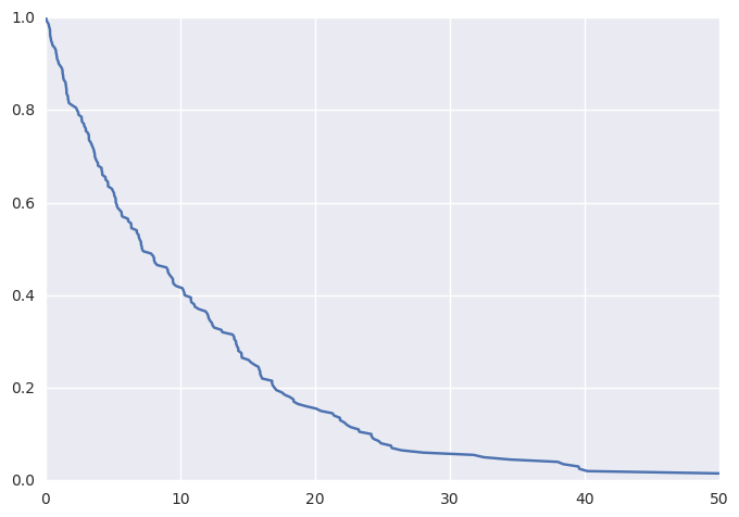
df = survivalstan.sim.sim_data_exp(censor_time = 50, N = 200, rate = 0.1)
Plotting these data (thanks to lifelines) as a KM curve yields
survivalstan.utils.plot_observed_survival(df, time_col='t', event_col='event')
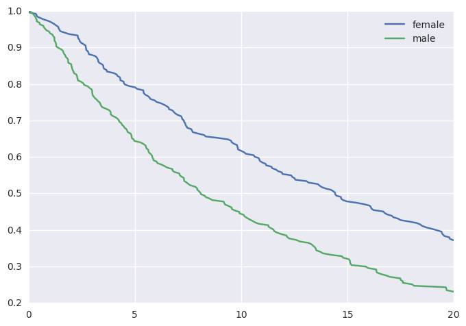
We can additionally simulate data where the hazard is a linear combination of covariate effects.
For example, where the hazard rate is a function of sex:
df2 = survivalstan.sim.sim_data_exp_correlated(
    N=500, censor_time=20, rate_form='1 + sex', rate_coefs=[-3, 0.5])
This would yield the following survival curves:
from matplotlib import pyplot as plt
survivalstan.utils.plot_observed_survival(
    df2.query('sex == "female"'),
    time_col='t',
    event_col='event',
    label='female')
survivalstan.utils.plot_observed_survival(
    df2.query('sex == "male"'),
    time_col='t',
    event_col='event',
    label='male')
plt.legend()
Fitting a Survival Model
We are now ready to fit our model to the simulated data.
To start with, we will fit a parametric exponential baseline hazard model – the same parameterization as we used to simulate our data:
fit1 = survivalstan.fit_stan_survival_model(
    df=df2,
    time_col='t',
    event_col='event',
    model_code=survivalstan.models.exp_survival_model,
    formula='~ age + sex',
    model_cohort = 'exp model'
)
Reviewing convergence
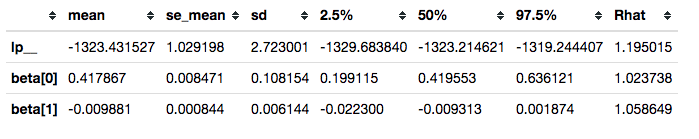
Summarizing posterior draws for key parameters, we see that the R-hat values are not great (R-hat is a rough indicator that your model is sampling well from the posterior distribution; values close to 1 are good):
survivalstan.utils.filter_stan_summary([fit1], pars=['lp__','beta'])
In some cases, it can be helpful to plot the distribution of R-hat values over the set of parameters estimated. This can help highlight parameters that are not being sampled well.
Updating the model
A trivial way to update a model is to increase the number of iterations:
fit2 = survivalstan.fit_stan_survival_model(
    df=df2,
    time_col='t',
    event_col='event',
    model_code=survivalstan.models.exp_survival_model,
    formula='~ age + sex',
    iter = 5000,
    chains = 4,
    model_cohort = 'exp model, more iter'
)
In the context of SurvivalStan, we use the parameter model_cohort to provide a descriptive label of either the model or the subset of data to which the model has been fit.
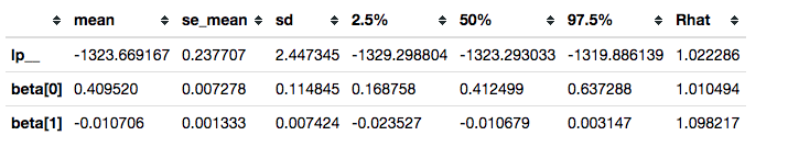
This is not sufficient to resolve our convergence problems.
survivalstan.utils.filter_stan_summary([fit2], pars=['lp__','beta'])
It is, however, good enough to illustrate our use case.
Summarizing posterior draws
You will notice that the functions above accept a list of fit objects, rather than a single fit object.
Most of the functions in SurvivalStan accept lists of models, since the typical modeling workflow is an iterative process.
For example, you can use the plot_coefs function to plot beta-coefficient estimates from one or several models:
survivalstan.utils.plot_coefs([fit1, fit2])
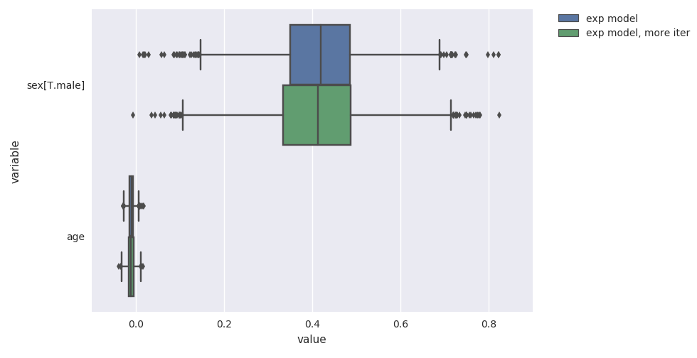
These are named/grouped according to the optional parameter model_cohort, which was provided when we fit the model.
Posterior predictive checks
SurvivalStan includes a number of utilities for model-checking, including posterior predictive checking.
This can be done graphically:
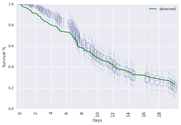
survivalstan.utils.plot_pp_survival([fit3], fill=False)
survivalstan.utils.plot_observed_survival(df=df2, event_col='event', time_col='t', color='green', label='observed')
plt.legend()
Or, posterior predictive summaries can be retrieved as a pandas dataframe. They are then available to be summarized or plotted more flexibly.
For example, in Test PEM model against simulated data.ipynb we demonstrate how to extract the predicted values and plot them using http://plot.ly:

Standard assumptions
We conclude this section introducing survival modeling by summarizing the key assumptions made by survival analysis, and their potential implications.
-
The most widespread assumption made by survival modeling is that the event will eventually occur for all patients in the study. The technique is called “survival modeling” because the classic endpoint of interest was death, which is guaranteed to happen eventually.
However, for many applications (e.g. disease recurrence or a purchase event) this assumption may not hold – i.e. some people may never purchase that product. In cancer research, where the goal is to eventually cure a significant portion of the population, we are starting to see portions of the population who are effectively “cured”, with near-zero disease recurrence risk up to 5 years following therapy. This is a good problem to have.
-
A second assumption is that the censoring is non-informative. Censoring can occur for many reasons – most often, and this is the best case, the study ends before all events are observed. In other cases, there is a competing event which leads to a patient being ineligible to continue in the study, or making it impossible to observe the primary clinical event. One example of a competing event in cancer research would be discontinuation of the drug due to toxicity. This type of event may be informative censoring, since the risk of the primary clinical event (i.e. mortality) may be different had the patient not experienced the toxicity.
In practice, violations of this assumption can be problematic to diagnose since outcome data for censored observations are rarely available. Gross violations of this assumption can directly affect utility and generalizability of the model estimates, particularly if the competing event is endogenous (i.e. related to treatment response or potential outcome). A common approach to address this problem is to estimate a competing risks model, in order to model the informative censoring process.
-
Finally, there is the proportional hazards assumption, which states that covariate effects on the hazard are uniform over the follow-up time. This is predominantly a simplifying assumption, which dramatically improves the ability to estimate covariate effects for smaller sample sizes. In practice, we often have biologically or clinically motivated reasons to think it may be violated. We will illustrate an example of this below.
More flexible baseline hazards
In addition to the assumptions noted above, we are also making a more obvious assumption that we have the right model – i.e. that our parameters are distributed as specified in the model.
When we simulate data, we have the confidence to know that our modeling assumptions aren’t violated. However, this can be difficult to determine in practice.
One of the more critical parameterizations to get right is that of the baseline hazard. The baseline hazard behaves like an intercept in a typical regression model. It describes the instantaneous hazard over time for the population in the absence of any covariate effects. Failure to get this right can lead to all sorts of pathologies whereby the excess variation in hazard not accounted for by your modeled baseline hazard will be absorbed into covariate effects, yielding invalid inferences and potentially misleading conclusions.
Aside: This is not a concern when using a Cox PH model for example, because the coefficient values are estimated using Maximum Likelihood Estimation (MLE) on a partial likelihood which does not include the baseline hazard. In a Bayesian analysis, however, we have the challenge of estimating the hazard as well as the coefficient effects.
Most of the time, we do not have a prior belief on the distribution of the baseline hazard. We usually do not care that much about what the features of the baseline hazard look like (although perhaps we should!). Instead, we are concerned with making sure our inferences about coefficient values are valid.
We thus want a baseline hazard that is sufficiently flexible to absorb any variation in the hazard over time which should not be attributed to covariate values. We also however want to minimize the risk of overfitting, so that our posterior predicted probabilities of survival are well calibrated. Many of the semi- or non-parametric approaches to modeling baseline hazards are very flexible with a penalty to impose the upper bound of complexity.
Piecewise hazards
Many non-parametric approaches to modeling the baseline hazard either implicitly or explicitly model the data using piecewise hazards. The most popular of these is the piecewise-exponential model (PEM).
Currently, to fit this model in SurvivalStan, you must provide data in long, denormalized, or start-stop format.
dlong = survivalstan.prep_data_long_surv(
    df=df2, event_col='event', time_col='t')
dlong['age_centered'] = dlong['age'] - np.mean(dlong['age'])
This breaks our survival time into blocks, such that we have at least one clinical event within each block. We end up with data where each patient has N records, one for each block in which the patient is still at risk for an event.
We can now fit this model using fit_stan_survival_model, in a manner similar to that used above.
fit3 = survivalstan.fit_stan_survival_model(
    model_cohort = 'pem model',
    model_code = survivalstan.models.pem_survival_model,
    df = dlong,
    sample_col = 'index',
    timepoint_end_col = 'end_time',
    event_col = 'end_failure',
    formula = '~ age_centered + sex',
    iter = 5000,
    chains = 4,
    )
Varying-coefficient models
Interaction effects are often biologically and clinically compelling results, and most detailed hypotheses imply the existence of one or several interaction effects. A search for predictive biomarkers often involves looking for biomarkers that interact with treatment, for example. And any hypothesis proposing that both X and K are required for benefit from treatment implies a three-way interaction.
However, interaction effects suffer from reduced power – the sample size required to detect an interaction effect is roughly 4-fold higher than that required to detect a main effect of similar magnitude with similar tolerance for type I and II error. And many of the exploratory biomarker analyses are underpowered for their main effects, in part due to expense and inconvenience of collecting biomarker data.
It can also be challenging to know, as an analyst, where to draw the line between searching for interaction effects which are biologically plausible, and mining the data for spurious “significant” findings. How to correct for multiple testing in this context? In any particular dataset, there are often a number of plausible interactions, some of which may yield significant findings by chance alone. Finally, parameter estimates within interaction subgroups can be unstable due to small numbers of subjects within combinations of groups.
A varying-coefficient analysis offers some of the benefits of interaction effects while mitigating (but not completely eliminating) the risks. It provides an intermediate ground between the two extremes of a full interaction, where effects are completely separate among groups, and no interaction, where effects are identical across groups. Instead, a varying-coefficient model results in what’s called partial pooling, where covariate effects can vary according to a group indicator, but only to the degree supported by the data and the model. Regarding the second point, in small sample sizes we often put a prior on the degree of variance across groups, reducing the likelihood for spurious interaction effects.
Example analysis
In an analysis we recently published, we included results from a varying-coefficient model. This analysis was conducted among a population of 26 patients with metastatic urothelial carcinoma treated with Atezolizumab, an anti-PD-L1 antibody. PD-L1 is a cell surface molecule that acts to suppress the anti-tumor activity of the immune system, so the hypothesized mechanism of drug action is to enhance the anti-tumor immune response by blocking this molecule’s binding to PD-1.
In this cohort, the response to the drug was higher among patients with high levels of PD-L1 expression on their tumor-infiltrating immune cells (IC2), than among patients with low or no detectable PD-L1 expression (IC1 and IC0, respectively). This makes biological sense – one would assume patients with PD-L1 expression would be more likely to respond to an anti-PD-L1 drug. What was surprising in this result is that there was also a response among the IC1 and IC0 patients, albeit at a lower level.
In this context, we hypothesized that mutation burden may also be associated with response, since mutated proteins provide the antigens recognized by the immune cells in their anti-tumor activity. In the absence of PD-L1 expression, mutation burden may be minimally associated with survival. In the presence of PD-L1 expression, however, patients with higher mutation burden may show an improved survival following therapy than patients with lower mutation burden.
We used SurvivalStan to fit a multivariate survival model where the coefficient that estimates the association of missense single-nucleotide variant (SNV) count per megabase (MB) with Progression-Free Survival could vary according to the level of PD-L1 expression.
Here are the results. This plot shows the estimated hazard ratio (HR) for Missense SNV Count / MB by PD-L1 expression level:
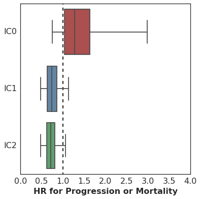
The association of mutation burden with Progression-Free Survival is highest (better survival with higher mutation burden) among patients with high PD-L1 expression (IC2), with lesser association among patients with lower levels of PD-L1 expression.
To fit this model using SurvivalStan, we used a model whose Stan code is archived with that repository but is now available in SurvivalStan as pem_survival_model_varying_coefs.
To fit it, you would use the following:
survivalstan.fit_stan_survival_model(
    df = df_long,
    formula = 'log_missense_snv_count_centered_by_pd_l1'
    group_col = 'pd_l1',
    model_code = survivalstan.models.pem_survival_model_varying_coefs,
    timepoint_end_col = 'end_time',
    event_col = 'end_failure',
    sample_col = 'patient_id',
    chains = 4,
    iter = 10000,
    grp_coef_type = 'vector-of-vectors',
    seed = seed
    )
See the analysis notebook on github for more details about this approach.
Time-dependent effects
For our next example, we will use one of the models provided by SurvivalStan which can estimate time-dependent effects.
Time-dependent effects occur when the hazard associated with a risk factor is not uniform over the entire follow-up period. In the context of clinical research, this can happen if a treatment or drug effect is delayed. In this case, the impact of the drug on survival may be minimal until t>X days after drug administration.
For example, consider the Kaplan-Meier curves reported in this NEJM paper reporting results from the Phase III trial of ipilumumab in a cohort of metastatic melanoma patients.
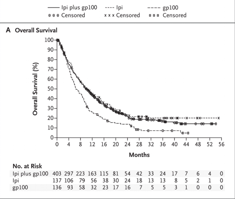
There is very little separation between Ipi-treated patients (ipi and ipi+gp100) cohorts and the control (gp100-only) cohort in the first 4 months. Only among patients surviving beyond the first 4 months do we see a difference in survival depending on the drug administered.
Now, this study was not analyzed using a time-dependent effects analysis, and for good reason - the goal of this analysis was to estimate the treatment effect overall in an intent-to-treat analysis. It’s important to keep your research goals in mind when considering an analysis.
There are cases where the analysis of time-dependent effects can be informative. For example, if you were looking to evaluate a potential predictive biomarker which could be used to identify which patients are likely to respond to treatment with ipilumumab, you may want to utilize the time-dependence of the treatment effect in your analysis.
For example
This is the strategy we took in our recent analysis of 26 patients with metastatic urothelial carcinoma treated with Atezolizumab. Like Ipilumumab, Atezo tends to show delayed treatment effect.
In this analysis, since we had such a small sample size, we hypothesized that there would be a sub-set of patients who were simply too sick to survive long enough to benefit from treatment; our collaborator called these the rapid progressors. In this subset, features like high mutational burden and a high level of PD-L1 expression – scenarios in which the drug is hypothesized to be particularly effective – wouldn’t matter since the drug wouldn’t likely be active at all. The prognosis of these patients would more likely be driven by their clinical status.
In effect, we hypothesized the existence of a time-dependent effect. Only among those patients who are healthy (or lucky) enough to survive long enough for the drug to be active, would the biomarkers like high mutation burden and high PD-L1 expression be relevant for slowing tumor progression & improving overall survival. As a rough estimate, our collaborator (who treats a number of patients with urothelial carcinoma) suggested 90 days as a cutoff.
Aside: As with all regression analyses, these models assume that your so-called “independent” covariates are exogenous – i.e. they are not a consequence of the treatment or the outcome. Biomarker values collected post-treatment are not typically exogenous, for two reasons: (1) patients have to survive long enough to have a measurement taken, and (2) such biomarkers are often intermediate measures affected by treatment & correlated with the outcome. These may indeed have time-dependent effects, but should be analyzed using a Joint Model.
The analysis
There are a few ways to “test” for time-dependent effects.
-
The first is to use the classical “test for non-proportional hazards”, which tests for non-zero correlation between scaled Schoenfeld residuals and time (or, log(time) since event times typically follow a poisson distribution). This test can be executed in R using cox.zph(). To my knowledge, there isn’t a python analog currently.
-
A second approach is to estimate time-dependent effects, and evaluate whether the HR is different over time for that biomarker. The evaluation can be quantitative (i.e. summarizing the max difference in HR over time for the biomarker), or qualitative (i.e. review graphical summary of time-dependent effects).
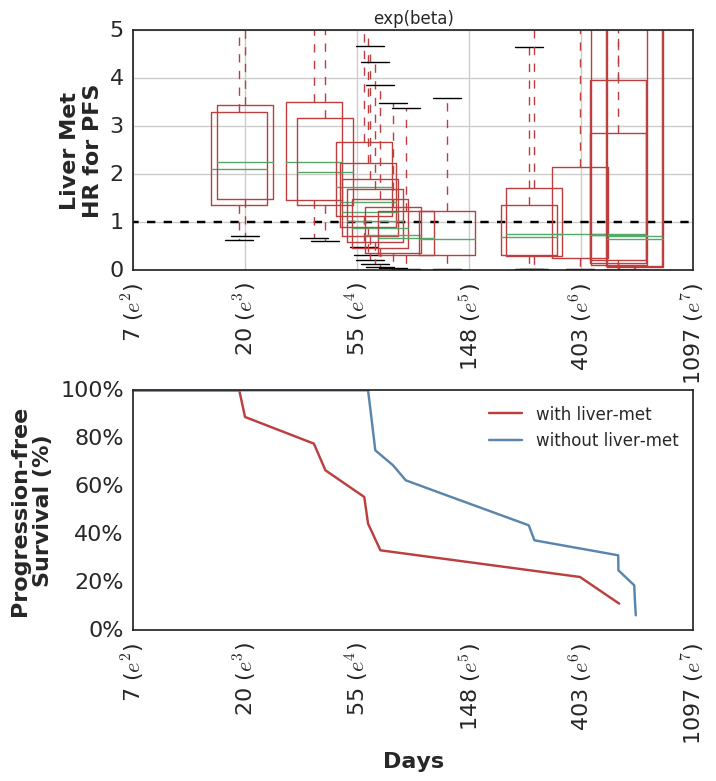
In our analysis, we started with the non-proportional hazards test in R (p = 0.04 for non-zero correlation of scaled Schoenfeld residuals with time) and then proceeded to estimate the HR for mutation burden separately for two intervals: [0 <= t <= 90d] and [90d >= t >= lastcensor].
Here are the estimated HR among all patients during the first 90d, and then among the subset of patients who remain in the cohort at t == 90d, looking only at events following 90d cutoff.
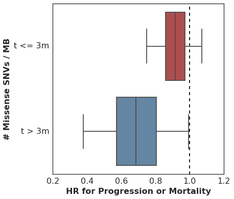
It’s worth pointing out that many analyses of cohorts similar to this one would drop these early failures from the analysis, since they did not survive long enough to benefit from therapy and thus are considered uninformative. This is problematic for several reasons, but most importantly it can overestimate the predictive value of the covariate alone. In practice, this detail in the sample selection is easy to overlook and a clinician would need to estimate the probability of an early failure in order to properly apply the biomarker’s predictive utility to a treatment decision.
At any rate, we then estimated the time-varying effect using a non-parametric analysis which models the association of mutation burden effect with survival as a random-walk over time.
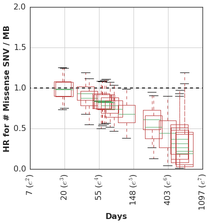
In this cohort, patients with higher mutation burden tend to have better survival, but only if they remain in the cohort long enough to see this benefit.
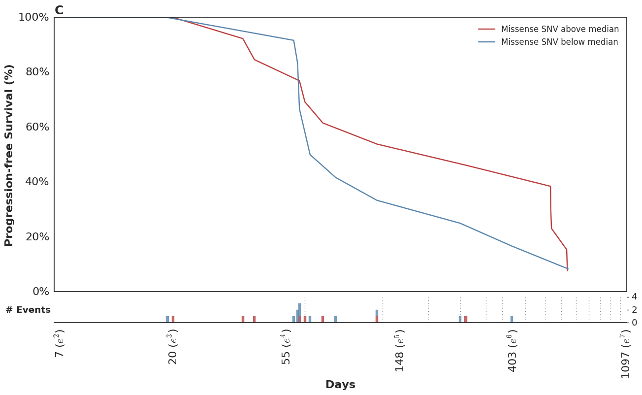
Looking at the posterior-predicted values by patients with high and low mutation burden, we can see the clear separation of the survival curves during the second half of the follow-up period:
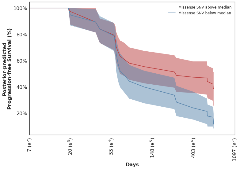
Which mirror the observed KM curves in this population.
In the course of this analysis, we fit this model using several parameterizations of the time-dependent effect. For more details, please refer to the complete analysis notebook in our github repo.
This wasn’t included in the original analysis, but we have subsequently looked at the clinical variables which were associated with higher risk of early failures. Not surprisingly, these show the inverse pattern of time-dependent hazards.
Fit using SurvivalStan
As with our previous example of varying-coefficient models, this model was fit using SurvivalStan.
fit = survivalstan.fit_stan_survival_model(
    model_cohort = 'time-dependent effect model',
    model_code = survivalstan.models.pem_survival_model_timevarying,
    df = dlong,
    sample_col = 'index',
    timepoint_end_col = 'end_time',
    event_col = 'end_failure',
    formula = '~ age_centered + sex',
    iter = 10000,
    chains = 4,
    seed = 9001,
    FIT_FUN = stancache.cached_stan_fit,
    )
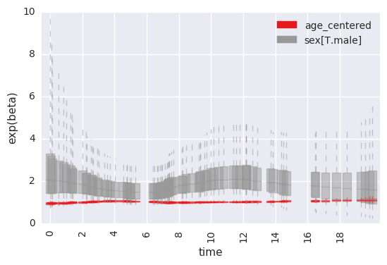
By default, all covariates included in the formula are fit with time-dependent effects. There is a weak prior on lack of time-variance for each parameter, and this can be edited by the analyst.
There are several utilities in SurvivalStan which support summarizing and plotting the posterior distributions of the parameters.
For example, to plot the time-specific beta coefficients (here, fit to simulated data with no time-dependent effects):
survivalstan.utils.plot_time_betas(models=[fit], by=['coef'], y='exp(beta)', ylim=[0, 10])
Conclusion
This concludes the first of what we expect to be several posts on Bayesian survival modeling. It demonstrates utilities of SurvivalStan for fitting a variety of Bayesian survival models using Stan, and allows the user to extend that set of models with a “Bring Your Own Model” framework.
More on this and other applications to come.
18 May 2017
| by
Tim O'Donnell
This post introduces a Python library called Kubeface for parallel computing on Google Container Engine using Kubernetes. We developed Kubeface to train the neural networks we publish in the MHCflurry package. There's nothing specific to neural networks in Kubeface, however, and we've used it to run a variety of compute-bound, easily-parallelized tasks.
Outline
Container engine background
Similar to Amazon Web Services (AWS) Elastic Compute Cloud, Google Compute Engine makes it easy to start and stop virtual machines, but leaves it to other systems to manage the deployment of jobs or services on these machines. Google Container Engine (GKE) addresses this need. It's a hosted deployment of Kubernetes, an open source project that grew out of Google infrastructure. Given a description of a service — for example, "run 5 database servers and 10 web servers" — Kubernetes starts, stops, and monitors the execution of docker images on Compute Engine instances to keep the service running.
Thanks to infrastructure support from the Parker Institute for Cancer Immunotherapy, we've been experimenting with Google Cloud as a platform for scientific computing.
Workload
Our neural network model selection task is an embarassingly-parallel problem in which we wish to train and evaluate a large of number neural network architectures. Each architecture evaluation runs on a single node. The data sizes are modest, at most a few gigabytes per model, but evaluating each model takes up to a few hours.
The table below shows the approximate design parameters for the jobs we need to run.
| Cluster size |
10-200 nodes (16-64 processors per node) |
| Simultaneously running tasks |
~200 |
| Time per task |
1 minute to 10 hours |
| Input size per task |
< 2 gb |
| Output size per task |
< 2 gb |
| Total tasks |
100 - 50,000 |
| Total time per job |
10 min - 10 days |
Existing solutions
In early experiments with Kubernetes, we quickly realized that some sort of layer between our application code and Kubernetes is required, as the the Kubernetes interface is too low-level and failure-prone to use directly as a job scheduler.
There are a number of projects in the Python ecosystem for farming out long-running tasks to remote workers, such as celery, dask.distributed, ipyparallel, and ray. On AWS, the PiCloud project was once popular but is no longer maintained. A recently developed package called PyWren that targets AWS Lambda looks promising, but is geared toward short-running jobs (300 seconds or less).
We initially experimented with celery (as described in this blog post) and dask.distributed to train our neural networks. With much-appreciated help from Matthew Rocklin, the author of dask.distributed, we succeeded in training the models released with MHCflurry 0.0.8 on GKE using this approach (see here for our configuration).
Systems like celery and dask.distributed have an architecture centered on persistent worker processes running on the worker nodes. The master dispatches tasks to the workers using a message queue (celery) or via a special scheduler process (dask). This approach has major advantages. Scheduled work can begin to run almost immediately, efficient inter-node communication patterns may be implemented, and the system is agnostic to the infrastructure used to start the workers (and is in fact a good fit for the service-oriented Kubernetes).
On the other hand, since the workers survive between tasks, state changed by one task can affect subsequent tasks in unforeseen ways, for example by creating temporary files that fill up the worker's disk. If a failure occurs, it can be unclear whether the problem is due to the master node, the scheduler, the worker node, or even a previous task run by the worker node. Debugging systems with distributed state and peer-to-peer communication is notoriously difficult. These packages also require a deployment process to launch the workers on the cluster. Each of our workloads require specific libraries installed in the Docker image, so we found ourselves starting and stopping deployments of dask.distributed workers frequently.
A simpler approach
A potentially better solution in our case is to schedule work directly on Kubernetes. We don't care about latency: in a multi-hour batch computation, it's fine if it takes a minute or two for a task to start running. While Kubernetes is designed for long running services, it provides some support for the sort of batch jobs that are common to scientific computing. We therefore came up with an approach in which tasks run in their own Kubernetes pods and all communication is done through Google Storage Buckets (the Google equivalent to Amazon's S3).
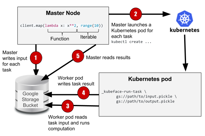
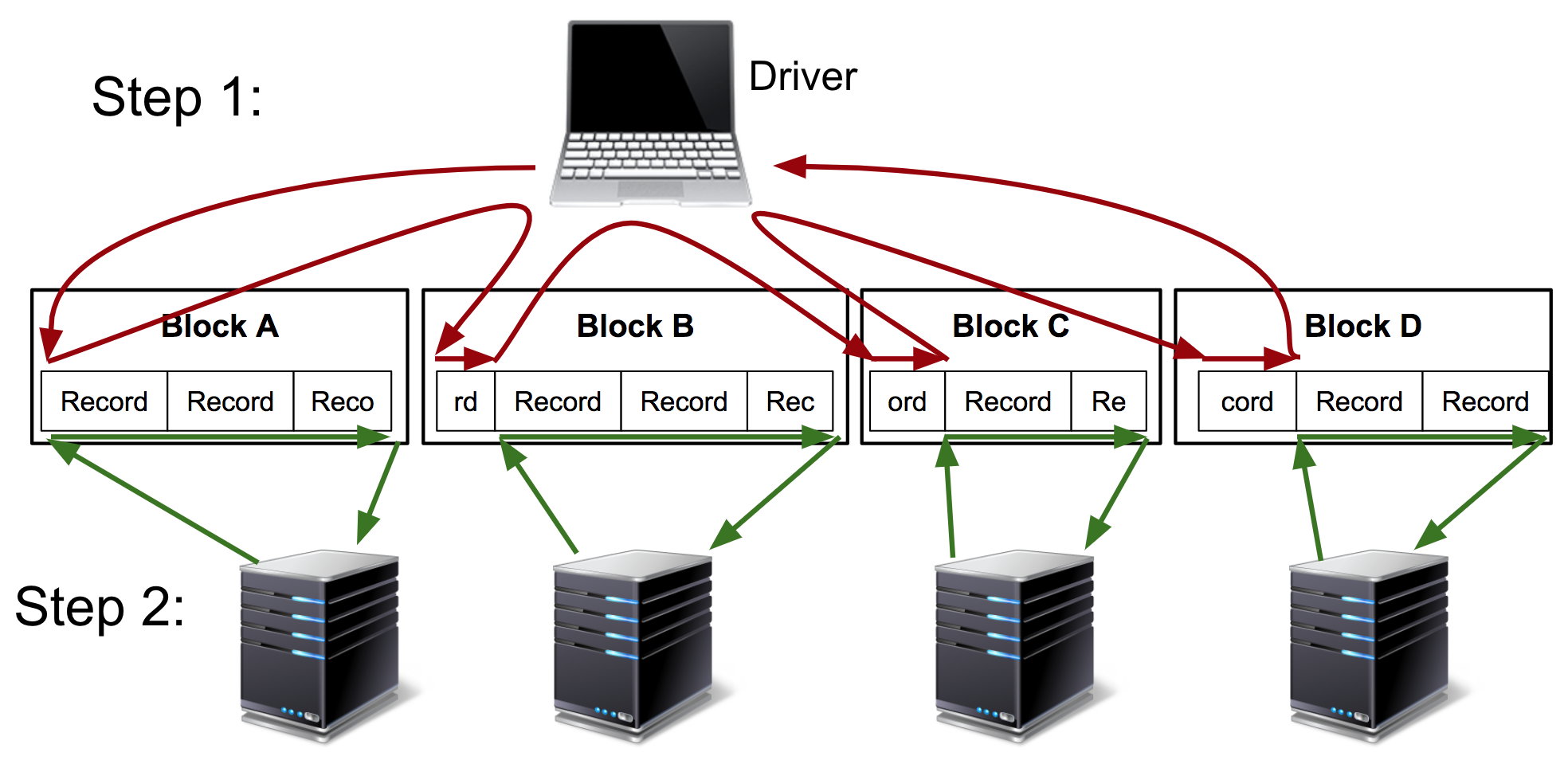
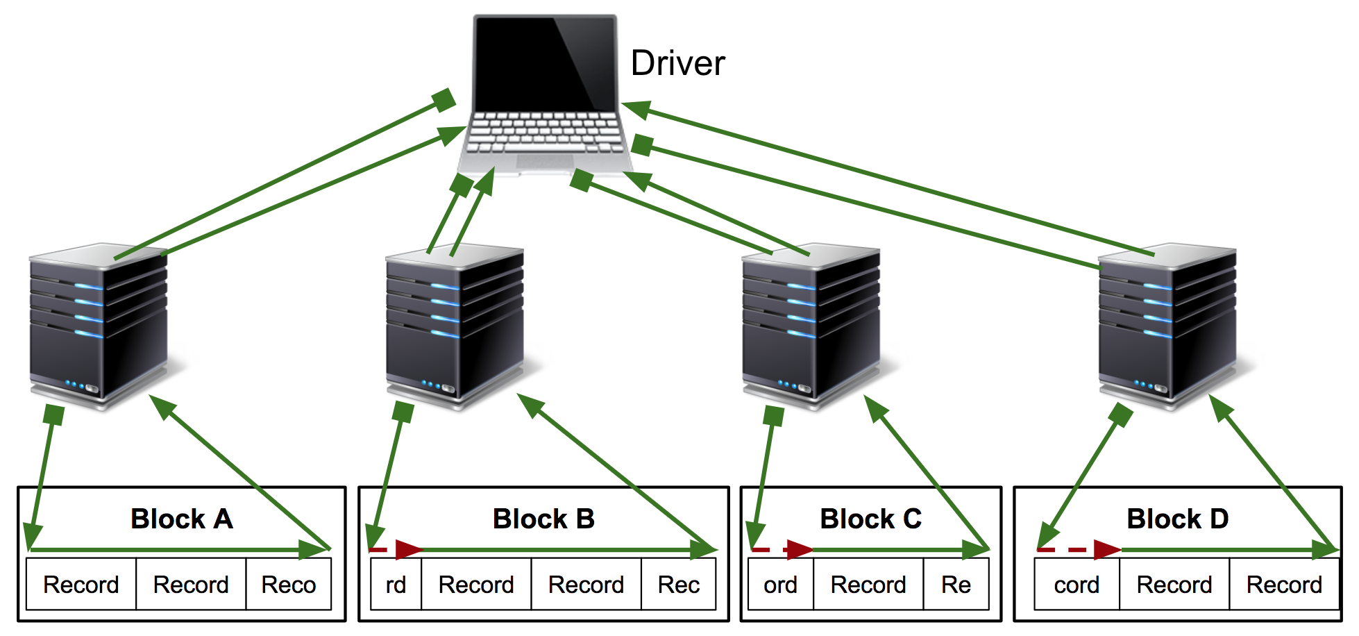
The Kubeface API is a parallel map. Kubeface invokes a function on each element in an iterable and returns the results. Each function invocation is called a task. As shown in the diagram, the Kubeface "master" process, i.e. the program the user runs, copies the input data for each task to the storage bucket. It then instructs Kubernetes to run pods that read the input data from the bucket, run the computation, and write the result to the bucket. The master process waits for the tasks to run and then reads the results from the bucket.
At the cost of some scheduling latency due to running a fresh Kubernetes pod for each task, as well increased I/O because we are moving data using a storage bucket instead of directly between nodes, we have a much simpler system. Tasks are isolated from each other, and a failing task may be debugged locally by invoking the Docker image. GKE supports auto-scaling clusters so we use only the instances we need. Importantly, the state of the distributed computation is simply the contents of the storage bucket. This simplifies debugging and also makes it straightforward to implement two useful Kubeface features: reuse of completed tasks when rerunning a failed job and speculative rerunning of straggling or failed tasks.
What’s next
We've used Kubeface to run several hundred jobs over the past three months, including MHCflurry model training and large analyses of the human proteome. While the system is increasingly reliable, debuggable, and performant we’ve hit plenty of issues. On the GKE side, we were surprised to find Kubernetes and Google Storage Buckets prone to transient service outages. Anywhere that Kubeface interfaces with these systems we've implemented a wait-and-retry policy. As Kubernetes seems to fail if we schedule more than 400 or so simultaneously running tasks, Kubeface must limit the number of tasks queued at once (we typically set the limit to 200). Kubernetes also loses the logs of pods frequently.
Aside from issues with GKE, the current Kubeface implementation itself leaves room for improvement. Most significantly, the Kubeface master does not track the progress of a task. It simply issues a call to Kubernetes to launch the task and then watches the storage bucket for the task's result to appear. A small number of task failures can be tolerated since speculation will cause dead tasks to be rerun eventually, but if a large number of tasks fail, the job will hang. It would be better to interface more tightly with Kubernetes and expose the status (e.g. pending, running, failed) to the master node. There are also a number of things we could do to improve the user experience, such as a more usable job status page and better handling of logs. In the longer term, it would be nice to support other Kubernetes deployments besides GKE, such as Kubernetes on Amazon EC2.
Kubeface is still early stage software, but we welcome anyone who would like to use or develop it further with us, as well as suggestions for better approaches. If you give it a try, check in and let us know how it goes!
16 May 2017
| by
Tim O'Donnell
We recently released an update to MHCflurry, our package for peptide/MHC binding affinity prediction. At a high level, MHCflurry is distinct from existing software in this space because it is:
- Developed in the open and licensed under the Apache 2.0 license
- Usable as a Python library or from the commandline
- Installable with the standard Python package manager
- Reasonably fast
- Re-trainable: users can fit their own data
In this post I’ll describe the problem MHCflurry solves and illustrate one approach we’re using to compare its performance to the popular NetMHCpan tool. Our benchmark suggests that our latest release is still not quite as accurate as NetMHCpan, but we’re getting close.
Outline
Immunology background
T cells patrol the body and kill any cells whose proteins are “abnormal” – for example, cells that are infected by a virus or cancerous. How the T cells establish what “abnormal” means here is a fascinating question that’s at the core of adaptive immunity, but we won’t be going into that topic in this post.
Proteins are mostly inside cells, so the T cells need a way to see what’s in there. Evolution’s solution to this, devised about 500 million years ago, requires cooperation from the monitored cells themselves. The proteins in a cell are subject to degradation (for eventual recycling) by the proteasome, a machine that chops proteins into small fragments, called peptides. The immune system takes advantage of this recycling system by shuttling some of the chopped up peptides onto a protein called MHC. The stuck-together peptide and the MHC, known as the peptide/MHC complex, is sent to the cell surface where it can be inspected by T cells.
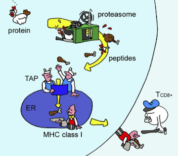 Antigen presentation. As proteins are degraded by the proteasome, some of the resulting peptides are trafficked to the endoplasmic reticulum (ER) where they are loaded onto MHC molecules and displayed on the cell surface. Figure from Yewdell, et al., Nature Reviews Immunology 2003.
Only a fraction of the peptides generated by the proteasome fit onto the MHC molecules, like a piece in a puzzle. This means that only certain peptides can elicit an immune response. What’s more, across the human population there are many variants (alleles) of MHC, each specific for a unique set of peptides. Thus the MHC-bound peptide repertoire (sometimes called the MHC ligandome) is in general different from one person to another.
When an MHC-bound peptide is recognized by a T cell, it’s called an epitope. Figuring out what the epitopes are in a protein is important in a lot of applications. For example, if you’re designing a vaccine to protect against a virus, it’s critical to include the epitopes from the viral proteins in the vaccine. Recently there’s been intense interest in understanding the epitopes arising from proteins mutated in cancer, known as neoantigens, since they seem to be responsible for much of the efficacy of immunotherapy.
Since binding MHC is a critical step for a peptide to be an epitope, many experimental techniques have been developed to determine whether an MHC molecule will bind a peptide. Purified peptides and MHC molecules can be assayed in vitro to measure how well they stick to each other, a quantity to known as binding affinity. Alternatively, peptide/MHC complexes can be stripped off cells and the peptides identified using mass spec. This gives a binary readout of the peptides bound to MHC. Experimental techniques like these have driven our understanding of immunology but require expensive equipment and specialized expertise.
Prediction algorithms
This is where machine learning tools like MHCflurry come in. MHCflurry is a collection of neural networks for predicting the binding affinity of a peptide and an MHC molecule. MHCflurry users can train predictors using their own affinity data (see the example notebook) or download models that we fit to measurements deposited in the Immune Epitope Database (IEDB). The latest MHCflurry includes 140 predictors, one for each MHC allele we support. Each of these predictors is an ensemble of 16 shallow artificial neural networks, themselves selected by grid-search over 160 model architectures. In total, we evaluated over 300,000 neural networks to generate the standard MHCflurry models, which required about 3.5 CPU years on Google Container Engine and motivated the development of Kubeface.
The standard tool for peptide/MHC binding prediction is NetMHCpan (Nielsen et al., Genome Medicine 2016), part of the NetMHC suite developed by Morten Nielsen’s group at Denmark Technical University. NetMHCpan is released as a closed-source binary that includes the model weights. The training data for NetMHCpan is not public; it uses the affinity data in IEDB combined with unspecified private data. Only the NetMHCpan authors can retrain it on new data. This makes it difficult to compare new predictors like MHCflurry against NetMHCpan, because one needs to generate an external validation set that NetMHCpan was not trained on, and NetMHCpan was trained on nearly all affinity data publicly available. An ongoing contest using data as it is submitted to IEDB enables some comparisons between tools but there are too few recent measurements for a reliable comparison.
Benchmarking with mass spec
Fortunately, recent advances have dramatically improved the accuracy and throughput of mass spec identification of peptides displayed on cell-surface MHCs. As we mentioned, in these experiments peptide/MHC complexes are stripped from cell surfaces. A mass spectrometer fragments the peptides into charged fragments, which are identified by their mass/charge ratio in a database search over the peptides present in human proteins. As this sort of data is not included in the training sets for MHCflurry or NetMHCpan, it’s a promising option to compare the performance of predictors trained on affinity data.
There’s a wrinkle, though. A mass spec result contains only positive examples – it’s a list of peptides that were found bound to MHC on a cell. Peptides not on this list could be missing for several reasons: proteins containing them may not have been expressed by the cell, the proteasome may not have cleaved them, or they may not have bound MHC. While it’s only the last case that constitutes a true negative example for our validation, from mass spec data alone we can’t differentiate these cases.
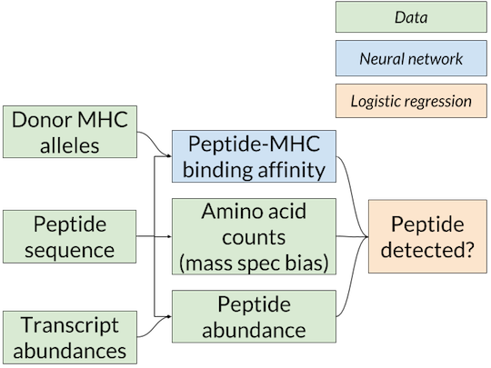 Nested-model scheme for benchmarking binding affinity predictors on mass spec data. A separate logistic regression model for each affinity predictor is trained and scored using that predictor’s affinity predictions. Since only the binding affinity predictor changes between logistic regression models, any differences in accuracy are due to the quality of the affinity predictions.
The solution we’ve adopted is the nested model shown above (similar to the one used in Abelin et al., Immunity 2017), in which the affinity predictions from MHCflurry or NetMHCpan are inputs to a logistic regression model that combines them with an estimate of the abundance of the peptide in the cell to give a final prediction on whether the peptide will be detected by mass spec. The abundance estimate comes from RNA-seq, which quantifies the messenger RNA present in a cell, and is thus a proxy for protein levels. We used RNA-seq from the cell lines used in the mass spec experiments or a similar cell type when this was not available. To train the logistic regression model, we choose random “decoys” from the proteome (not detected by mass spec) to constitute our negative examples.
Two technical notes: first, as certain amino acids (especially cysteine) may be under-represented in mass spec datasets due to their chemistry, we also include the counts of each amino acid in the peptide to the logistic regression model. This allows it to learn amino acid biases of the mass spec assay. Second, in other experiments, we have also incorporated proteasomal cleavage predictions, but the results do not change qualitatively so for simplicity we are omitting that from this post.
We evaluated four affinity models using this approach:
- NetMHCpan 3.0
- single-network MHCflurry models trained on IEDB (released in MHCflurry 0.0.8)
- ensemble-network MHCflurry models trained on IEDB (released in MHCflurry 0.2.0),
- an experimental MHCflurry model trained on mass spec (unreleased)
We’re including the last predictor as an interesting example of potential next steps. This predictor is trained on mass spec data, not affinity measurements like the others.
To train the logistic regression models (as well as the experimental mass spec-based affinity model), we used the mass spec hits published in Abelin et al., Immunity 2017 from a B cell line. We then scored the predictors on the four experiments in HeLa cell lines (each with a single MHC allele) from Trolle et al., Journal of Immunology 2016 as well as the peripheral blood mononuclear cells (PBMC) from Caron et al., eLife 2015. The training and testing data come from different labs, experimental conditions, and cell types. In this analysis we are considering only length 9 peptides, the most common length of MHC-binding peptides.
To score the predictors, we ranked all peptides in the proteome by the logistic regression model’s output, then calculated the positive predictive value (PPV) of the models at a very a stringent threshold (specifically, we calculated the fraction of the top N predicted-peptides that were observed in the mass spec hits, where N is the number of mass spec hits).
Results
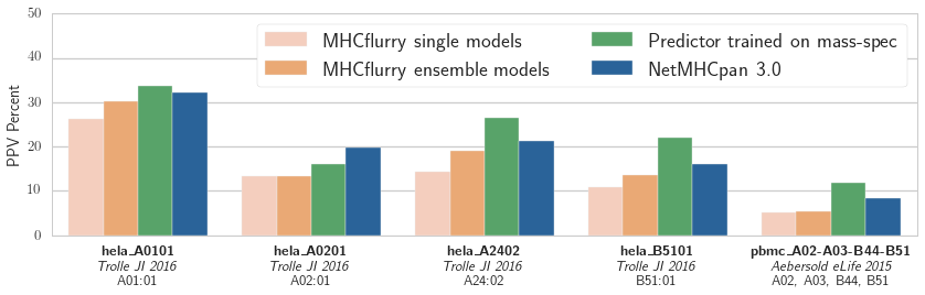 Positive predictive value (PPV) of the logistic regression models associated with each binding affinity predictor over five validation datasets from two publications. The training data was from the independent mass spec dataset published in_ Abelin et al, Immunity 2017
Our results are shown in the figure. The NetMHCpan-based predictor outperforms both MHCflurry predictors trained on IEDB data. We have more work to do! We also see that the experimental predictor trained on mass spec performs best. This is interesting, as the mass spec training data is smaller than the IEDB affinity data (about 1,000 mass spec hits per experiment compared to about 4,000 measurements in IEDB for each of these alleles). While some of this may be due to subtle biases in mass spec detection (which may be learned by the predictor), it’s encouraging evidence that relatively small amounts of mass spec data may enable a substantial improvement in affinity prediction.
Going forward, we are working on training MHC affinity predictors that can learn from both affinity measurements and mass spec data to make the best predictions possible. With any luck we’ll be updating you on those developments soon!