At Hammer Lab, we use Spark to run analyses of genomic data in a distributed fashion. Distributed programs present unique challenges related to monitoring and debugging of code. Many standard approaches to fundamental questions of programming (what is my program doing? Why did it do what it did?) do not apply in a distributed context, leading to considerable frustration and despair.
In this post, we’ll discuss using Graphite and Grafana to graph metrics obtained from our Spark applications to answer these questions.
Graphs of various metrics about the progress of a Spark application; read on for more info.
Spark Web UI
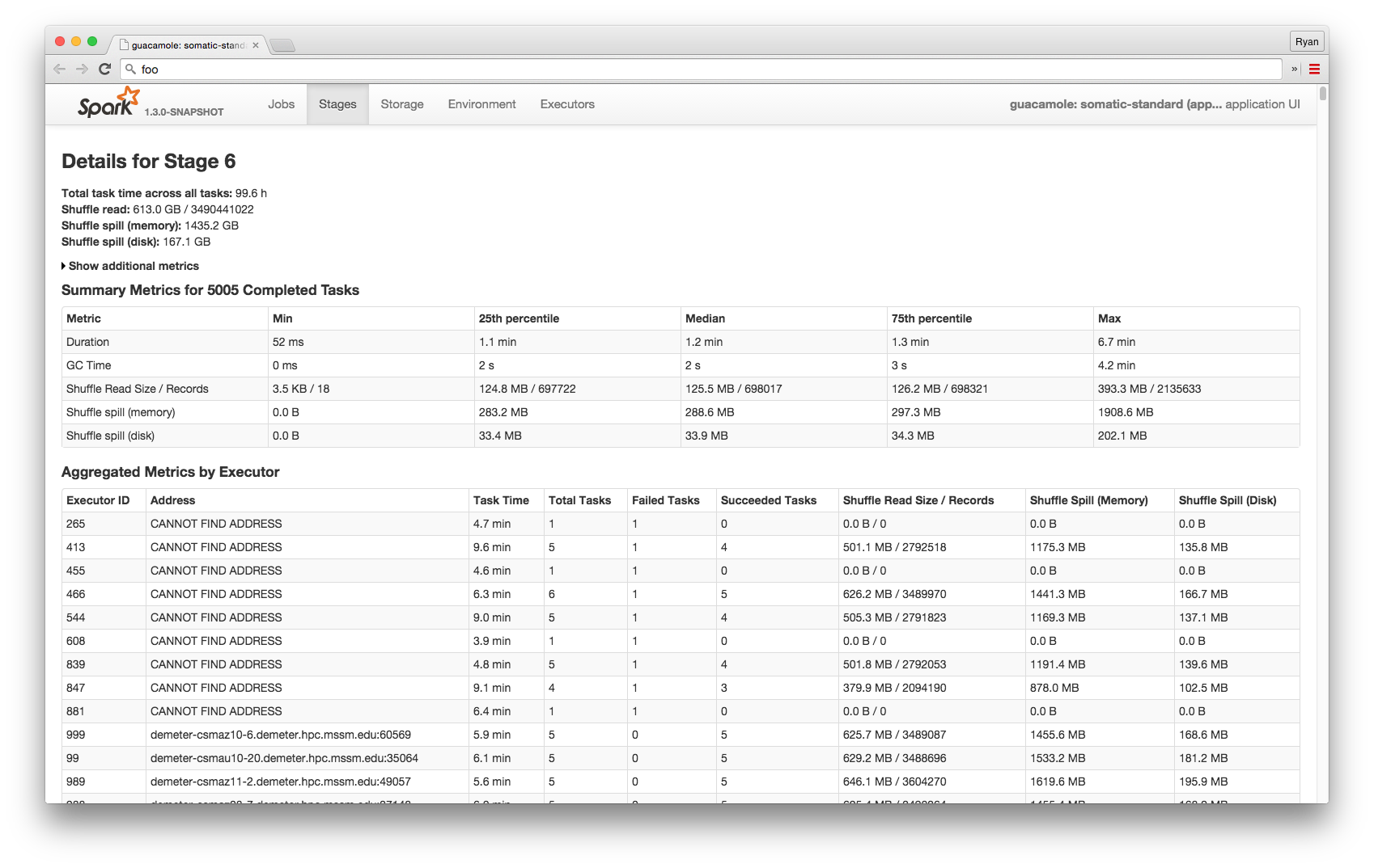
Spark ships with a Jetty server that provides a wealth of information about running applications:
Here we see a page with information about a specific stage in a job: completed tasks, metrics per executor, and (below the fold) metrics per task.
This interface seems to be the way that most users interact with Spark applications. It gives a good overview of the state of an application and allows for drilling into certain metrics, such as bytes read from HDFS or time spent garbage collecting.
Buried in a rarely-explored corner of the Spark codebase is a component called MetricsSystem. A MetricsSystem instance lives on every driver and executor and optionally exposes metrics to a variety of Sinks while applications are running.
In this way, MetricsSystem offers the freedom to monitor Spark applications using a variety of third-party tools.
Graphite
In particular, MetricsSystem includes bindings to ship metrics to Graphite, a popular open-source tool for collecting and serving time series data.
This capability is discussed briefly in the Spark docs, but there is little to no information on the internet about anyone using it, so here is a quick digression about how to get Spark to report metrics to Graphite.
Sending Metrics: Spark → Graphite
Spark’s MetricsSystem is configured via a metrics.properties file; Spark ships with a template that provides examples of configuring a variety of Sources and Sinks. Here is an example like the one we use. Set up a metrics.properties file for yourself, accessible from the machine you’ll be starting your Spark job from.
The --files flag will cause /path/to/metrics.properties to be sent to every executor, and spark.metrics.conf=metrics.properties will tell all executors to load that file when initializing their respective MetricsSystems.
Grafana
Having thus configured Spark (and installed Graphite), we surveyed the many Graphite-visualization tools that exist and began building custom Spark-monitoring dashboards using Grafana. Grafana is “an open source, feature rich metrics dashboard and graph editor for Graphite, InfluxDB & OpenTSDB,” and includes some powerful features for scripting the creation of dynamic dashboards, allowing us to experiment with many ways of visualizing the performance of our Spark applications in real-time.
Examples
Below are a few examples illustrating the kinds of rich information we can get from this setup.
Task Completion Rate
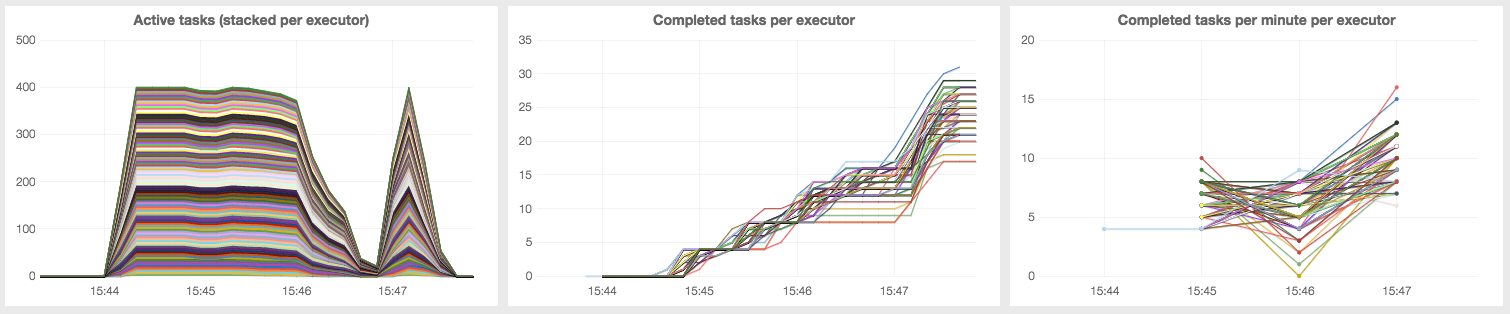
These graphs show the number of active and completed tasks, per executor and overall, from a successful test of some toy read depth histogram functionality in a branch of our Guacamole variant calling project:
The leftmost panel shows close to 400 tasks in flight at once, which in this application corresponds to 4 “cores” on each of 100 executors. The “valley” in that leftmost panel corresponds to the transition between two stages of the one job in this application.
The right two panels show the number of tasks completed and rate of task completion per minute for each executor.
HDFS I/O
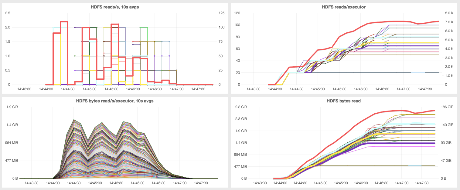
MetricsSystem also reports all filesystem- and HDFS-I/O at per-executor granularity. Below are some graphs showing us our application’s HDFS read statistics:
Clockwise from top left, we see:
a peak of ~100 HDFS reads per second (red line, right Y-axis), with individual executors topping out around ~2/s over any given 10s interval (thinner multi-colored lines),
a total of ~700 HDFS reads (red line, right Y-axis) over the application’s lifespan, with individual executors accounting for anywhere from ~20 to ~100,
a total of ~180 GB of data read from HDFS (red line, right Y-axis), which is in line with what was expected from this job, and
a peak total read throughput of around 1.5 GB/s.
Our applications are typically not I/O bound in any meaningful way, but we’ve nonetheless found access to such information useful, if only from a sanity-checking perspective.
JVM
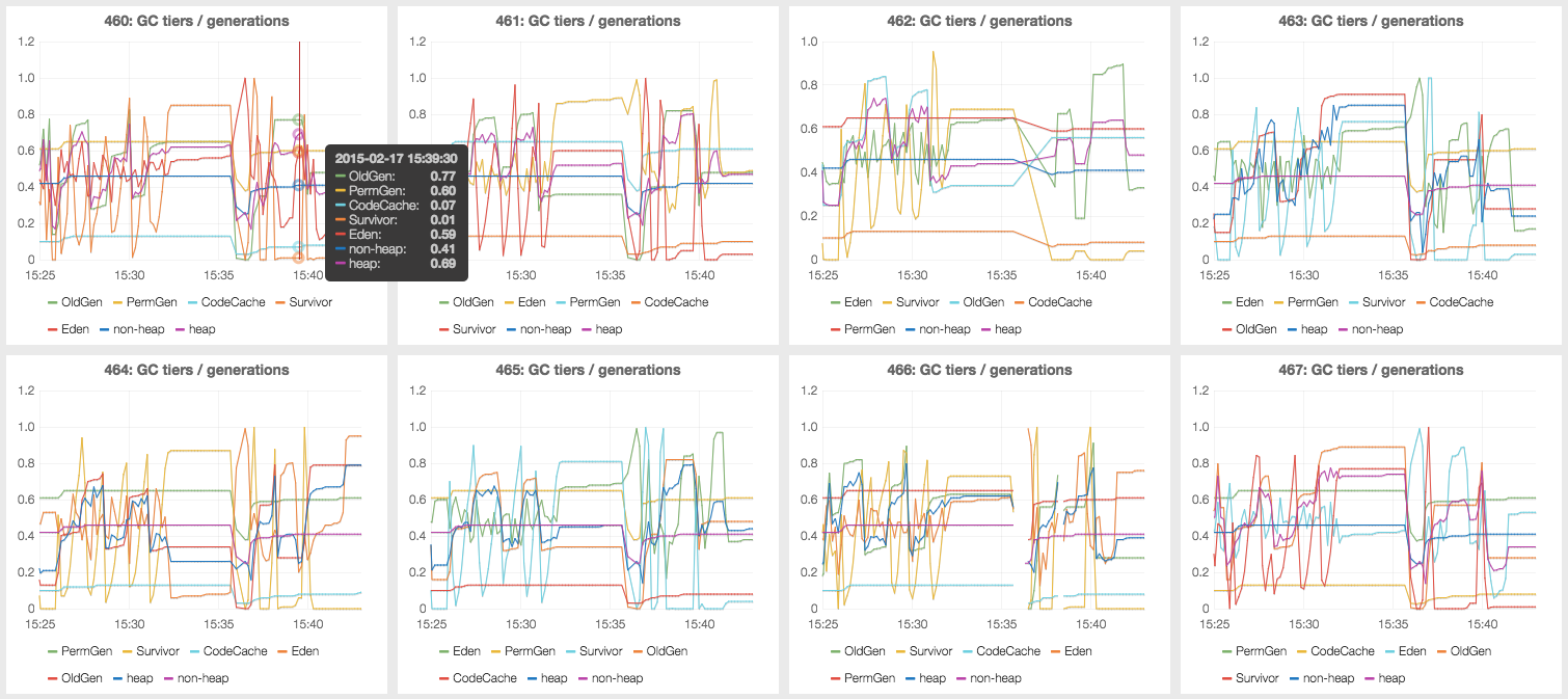
The JVM statistics exported by Spark are a treasure trove of information about what is going on in each executor. We’ve only begun to experiment with ways to distill this data; here’s an example of per-executor panels with information about garbage collection:
Let’s do some forensics on a recent failed run of our SomaticStandard variant caller and use our Grafana dashboard to diagnose an issue that proved fatal to the application.
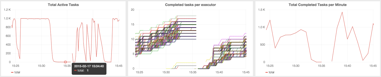
The graphs below, similar to those in the first example above, show the number of active and completed tasks, per executor and overall, during a period in the middle of the doomed application’s lifetime:
From experience, we have learned to note and infer several things from graphs like these:
All three graphs have a discontinuity toward the middle of the time window presented here.
This is likely due to the application master (AM) restarting.
Related: all “completed tasks per executor” (middle panel) counts restart from zero when the new AM spawns new executors.
In the lead-up to the discontinuity / AM restart, forward progress had almost completely stopped.
The tooltip on the left graph shows that there were several minutes where only one task (and therefore executor) was active (out of 1000 total executors).
The “completed task” counts in the right two graphs show no movement.
Finally, there are a suspicious couple of new lines starting from 0 in the middle graph around 15:31-15:32.
Why are executors coming to life this late in the application?
Answer: these new executors are replacing ones that have been lost.
Something during this flat-lined period is causing executors to die and be replaced.
Putting all of this information together, we conclude that the issue here was one of a “hot potato” task inducing garbage collection stalls (and subsequent deaths) in executors that attempted to perform it.
This is a common occurrence when key skew causes one or a few tasks in a distributed program to be too large (relative to the amount of memory that has been allocated to the the executors attempting to process them). The study of skew in MapReduce systems dates back to the earliest days of MapReduce at Google, and it is one of the most common causes of mysterious Spark-job-degradation-or-death that we observe today.
As usual, we’ve open-sourced the tools showcased here in the hopes that you’ll find them useful as well. The hammerlab/grafana-spark-dashboards repo contains a script that you should be able to use off-the-shelf to bootstrap your own slick Grafana dashboards of Spark metrics.
Future Work
The development and standardization of sane tools for monitoring and debugging Spark jobs will be of utmost importance as Spark matures, and our work thus far represents only a tiny contribution toward that end.
Though the grafana-spark-dashboards previewed above have been useful, there’s still an ocean of relevant data we would love to get out of Spark and onto our graphs, including but not limited to:
Structured information about jobs and stages, particularly start-/end-times and failures.
Information about what host each executor is running on.
Task- and record-level metrics!
Spark #4067 added such metrics to the web UI, and it would be great to be able to see them over time, identify executors / tasks that are lagging, etc.
Reporting task failures, even one-offs, would be useful; it is sometimes surprising to behold how many of those occur when perusing the logs.
In addition, supporting other time series database or metrics collection servers (e.g. StatsD, InfluxDB, OpenTSDB) would open up more avenues for users to monitor Spark at scale.
We hope this information, as well as the grafana-spark-dashboards starter code, will be useful to you; happy monitoring!
In this post we’ll set up continuous testing on Travis-CI. We’ll also take
advantage of our Mocha testing setup to track code coverage on every
build.
If you want to skip straight to the finished product, check out this
repo.
Running Tests on Every Commit
Tests are more effective when they’re run on every commit, allowing for a clear
association between each test failure and the commit at fault.
The easiest way to do this for a GitHub project is with Travis-CI. To set this
up, create a .travis.yml file like this one file and enable
your project at travis-ci.org.
Why Code Coverage?
Running your tests on every commit is helpful, but how do you know that you’ve
written enough tests? One way to answer this question is with code
coverage, which tells you which lines of your code are executed by
your tests.
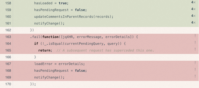
(The red lines show that the failure case is untested.)
Code coverage can help guide your test writing. If one branch of an
if statement is covered but the other isn’t, then it’s clear that you need to
write a new test.
Writing tests isn’t always the most fun part of software development. Tracking
test coverage over time adds a dash of gamification to the
process: it can be motivating to watch the coverage percentage go up!
Generating Code Coverage Data
Generating code coverage data can be fairly involved. It requires instrumenting
your code with counters that track how many times each line is executed. In
fact, we don’t know of any way to do this for Jest tests, which we
used before switching to Mocha. It’s also hard to generate
coverage data with Mocha, but here we get to benefit from its extensive
ecosystem: someone has already done the hard work for us!
We used Blanket to instrument our code for coverage:
npm install --save-dev blanket glob
We also had to add a blanket config section to our package.json:
blanket-stub-jsx.js is a custom compiler that we had to
write. As before, our decision to use JSX, Harmony and stubs has
simplified our code but made the processes that operate on our code more
complicated. This is a trade-off.
The "pattern": "src" tells Blanket where to find modules to instrument for
coverage. If you don’t specify this, only files which are explicitly included
by your tests will contribute to coverage. Untested files won’t count. Telling
Blanket about them will reduce your test coverage percentage, but at least
you’re being honest. And it will encourage you to write more tests for those
untested files to bring that percentage back up!
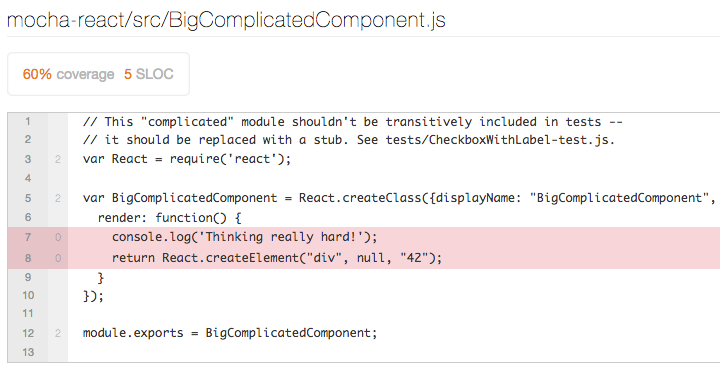
Mocha includes a few “reporters” for displaying code coverage data. One of
these is html-cov, which will generate an HTML page summarizing your code
coverage:
(A web view of test coverage for BigComplicatedComponent.js. Note that this is
the compiled code, not our original JSX/Harmony code. More on that below.)
Much like the tests themselves, code coverage works best when you track it on
every commit. If you don’t, coverage might drop without your realizing it.
coveralls.io is a test coverage site which is free for open source
projects and integrates nicely with GitHub and Travis-CI. So long as you can
produce coverage data in the correct format, coveralls will track the changes in
your project’s test coverage, generate badges for your project and provide a
nice test coverage browser.
Coveralls works best when you send it coverage data directly from a
Travis worker. To set this up we installed a few NPM packages…
Here’s what the code coverage data looks like on coveralls:
(Coverage of BigComplicatedComponent. Note that its render method is never
called, because it’s stubbed in the test.)
It’s worth noting that coverage is measured on the transpiled JavaScript code,
but displayed against the original code on Coveralls. This only works because
the JSX/Harmony compiler preserves line numbers.
Conclusions
Continuous code coverage is one of the big wins of using Mocha to test React apps. It takes a bit of work to set up, but the motivation it gives you to write more tests is well worth the effort.
If you have any issues or ideas regarding this setup, please file an issue on our example repo.
Unit testing is an essential part of software engineering. Tests provide living
documentation of expected behaviors, prevent regressions, and facilitate
refactoring. Web applications benefit from testing as much as any other kind of
software.
In recent years there’s been a proliferation of JavaScript frameworks and
testing tools. Piecing together a combination of tools that works well can be
daunting. We use React.js components in CycleDash, so in this post I’ll
describe our usage of Mocha for testing React with JSX and ECMAScript 6 (Harmony).
If you want to skip straight to using the setup described here, check out this
repo. There’s also a follow-up post which talks about
generating code coverage data.
How About Jest?
Facebook recommends using Jest for testing React apps. Jest
is a testing framework based on Jasmine that adds a few helpful features
for testing React-based applications:
We used Jest for a few months, and it certainly makes it easy to start writing tests for React apps. That said, we ran into some pain points and missing features:
Cryptic error messages.Long stack traces that are missing important
information.
Incompatibilities. For example, there was some kind of problem
with Jest and contextify, a widely-used node.js library. D3 required
jsdom, which required contextify, so we couldn’t test D3 components with
Jest.
Slow test execution. Startup time was particularly bad. It was common to
wait 5-10 seconds for a single test to run.
We also began to realize that, while auto-mocking reduces test dependencies and can result in faster and more “unit-y” tests, it can have some negative consequences. What if you factor a sub-component out into its own module? Or extract a utility library? The API and behavior of your code is unchanged, but auto-mocking will make all of your tests break. It exposes what should be an implementation detail. And, because Jest mocks modules by making all their
methods return undefined, this usually manifests itself in the form of cryptic errors stating that undefined is not a function.
Setting Up Mocha
Once we decided to use another testing framework, we considered Mocha, Jasmine, and QUnit. Because we were using node-style require statements, QUnit wasn’t a natural fit. Mocha is widely used and appears well supported, so we decided to run with it.
While it is very easy to get up and running with React testing using Jest, doing the same with
Mocha is a bit more involved. To get our tests to run, we had to
re-implement a few of its perks: DOM mocking, JSX transpilation and (opt-in) module mocking.
This snippet needs to go before React is required, so that it knows about
the fake DOM. You could probably get away without setting global.navigator,
but we found that some libraries (e.g. D3) expected it.
JSX Transpilation
In any React.js project, you need to make a decision about whether to use JSX
syntax. There are good reasons to go either way. We decided to
use JSX and so we needed to adjust our test setup to deal with this. Having to
do this is one of the downsides of JSX. It simplifies your code, but it
complicates all the tools that work with your code.
To support JSX with Mocha, we used a Node.js “compiler”. This is a bit of
JavaScript that gets run on every require. It was originally created to
facilitate the use of CoffeeScript, but it’s since found other uses as the set
of “compile to JS” languages has expanded.
We based our compiler on this one from Khan Academy:
// tests/compiler.jsvarfs=require('fs'),ReactTools=require('react-tools'),origJs=require.extensions['.js'];require.extensions['.js']=function(module,filename){// optimization: external code never needs compilation.if(filename.indexOf('node_modules/')>=0){return(origJs||require.extensions['.js'])(module,filename);}varcontent=fs.readFileSync(filename,'utf8');varcompiled=ReactTools.transform(content,{harmony:true});returnmodule._compile(compiled,filename);};
Our compiler is slightly more complex than the Khan Academy compiler because we
don’t use a .jsx extension to distinguish our React code. As such, we need to
be more careful about which modules we process, lest the JSX compiler slow down
our tests.
To use this compiler, you pass it via the --compilers flag to mocha:
The . indicates that the compiler should run on files with any extension. If
you consistently end your JSX files with .jsx, you can specify that instead.
Our preprocessor also enables ECMAScript 6 transpilation. This lets
you use some of the nice features from the upcoming JS standard like function arrows,
compact object literals, and destructuring assignments. If you’re going to go
through the trouble of enabling JSX transpilation, there’s really no downside
to enabling Harmony and there’s a lot of upside.
You can find a version of the Jest/React demo using this setup in this repo.
Mocking/Stubbing Components
While auto-mocking modules has undesirable consequences, explicitly stubbing
out React components can lead to faster, more isolated tests. Note that
we’ll use the term “stub” from here on out instead of “mock.”
We initially tried to implement stubbing using proxyquire, but we ran into fundamental issues relating to the node package cache. If a module was stubbed the first time it was required, it would continue to be stubbed on subsequent requires, whether this was desirable or not. Disabling the cache led to poor performance.
We concluded that this was a job best done, again, by a node compiler. When a module is “compiled”, we check whether it’s in a whitelist of modules which should be stubbed. If so, we stub it. Otherwise, we transpile it as usual.
We tried to be smart about stubbing the precise API of each module (like Jest does). But this turned out to be harder than expected. After banging our heads against the problem, we realized that everything we’d want to mock was a React component. And React components all have simple, identical APIs. So we simplified our stubbing system by only allowing React components to be stubbed.
Here’s what the usage looks like:
require('./testdom')('<html><body></body></html>');varReact=require('react/addons');global.reactModulesToStub=['BigComplicatedComponent.js'];// When HighLevelComponent does require('BigComplicatedComponent'),// it will get a stubbed version.varHighLevelComponent=require('HighLevelComponent');
Supporting this makes the compiler a bit more complex. Here’s the gist of it:
// A module that exports a single, stubbed-out React Component.varreactStub='module.exports = require("react").createClass({render:function(){return null;}});';functiontransform(filename){if(shouldStub(filename)){returnreactStub;}else{varcontent=fs.readFileSync(filename,'utf8');returnReactTools.transform(content,{harmony:true});}}
Note that this assumes that each React Component lives in a separate module
which exports the Component. For larger applications, this is a common pattern.
You can find a fully-worked example using JSX and stubs in this repo.
Using Mocha
Now that we’ve added support for JSX/Harmony and module stubbing to Mocha, we can take advantage of all of its features and addons. We’ll walk through a few testing essentials.
To run just a single file of tests, pass it as the last argument. You can also
pass --grep <test regex> to run a subset of a file’s tests. To run the
version of mocha specified in your package.json file, use
node_modules/.bin/mocha instead.
Mocha is considerably faster at executing a single test from the command line
than Jest. For the simple Jest example test, execution time on my machine
dropped from 1.65s to 0.138s, a 12x speedup. For projects with many tests,
those seconds add up.
Debug Tests in a Browser
Most browsers provide comprehensive JavaScript debugging tools. If you don’t
use these tools, you’re making your life harder! The inability to run Jest
tests in-browser was one of the reasons we switched to Mocha.
Mocha tests typically use require statements and often access the file
system, so running them directly in the browser is challenging. The next best
thing is to use node-inspector, which connects a version of the Chrome
dev tools to the Node runtime used by Mocha.
Then run node-inspector. It will prompt you to open a browser at a debug URL.
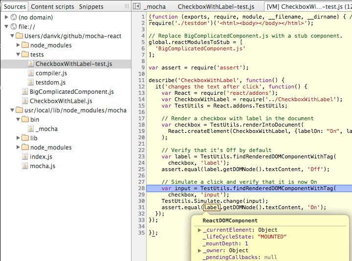
From there, you can set breakpoints and inspect variables in the same way you
would in the Chrome Dev Tools:
(Debugging a React/Mocha test with node-inspector. Note that this is transpiled code.)
Conclusions
Testing a React app with Mocha does require some extra plumbing, but we
ultimately found the transition to be well worth the effort.
There are more advantages to using Mocha than just the ones we’ve discussed in this post.
In the next post, we’ll talk about how we generate test coverage on
every commit.
We hope that this post helps you find your way to the same happy testing place we have found!
Last week we introduced our Spark-based variant calling platform, Guacamole. By parallelizing over large clusters, Guacamole can identify mutations in a human genome in minutes, while comparable programs typically take hours.
Guacamole provides a set of primitives for distributed processing of DNA sequencing data. It also includes a few proof of concept variant callers implemented using these primitives. The GermlineStandard variant caller identifies differences in a sample with respect to the reference genome, commonly referred to as germline variants. Germline variant calling can discover mutations that might cause a congenital disorder. The SomaticStandard caller is for cancer studies and identifies mutations that occur in a patient’s cancer cells but not in his or her healthy cells.
SomaticStandard
Similar to many other variant callers, we use a simple likelihood model to find possible variants, then filter these to remove common sources of error.
The input to a variant caller is a collection of overlapping reads, where each read has been mapped to a position on the reference genome. In addition, the sequencer provides base qualities, which represent the machine’s estimate of a read error. For example:
chr1 724118 AATAAGCATTAAACCA @B@FBF4BAD?FFA
where AATAAGCATTAAACCA is positioned at chr1, position 724118, and the sequencer provided the error probabilities @B@FBF4BAD?FFA. Each letter represents a Phred-scaled probability of the sequencer having correctly identified the corresponding base.
This read and others that overlap position 724118, collectively referred to as a “pileup,” can be used to determine the genotype at that position. A genotype is the pair of bases, one from each parent, that an individual has at a particular location in the genome. We can compute the posterior probability of each possible genotype, given the observed reads, using Bayes’ Rule. For example, if R is the collection of reads that overlap position p and AT is the genotype we want to evaluate:
We compute the likelihood
(i.e. how likely is it that we would see this collection of reads if the patient truly had one chromosome with an A and one with a T at this position) using the base qualities. We assume that each read is generated independently:
Then, if is the probability of a sequencing error on read i at this position:
We consider the tumor and normal samples independently at each position and compute the likelihood that the tumor has a different genotype than the normal tissue, indicating a somatic variant.
This likelihood model is simple and highly sensitive, but it ignores important complicating factors that contribute to false positive variants. For example, Illumina sequencing machines have well-documented issues toward the beginning and end of reads and sometimes sample one DNA strand more frequently than the other. Additionally, reads in high-complexity regions may be misaligned by the aligner. A number of filters are applied to remove erroneous variants due to these factors.
Improvements
Errors in variant callers tend to come from three main areas:
Guacamole will correct sequencing errors through the examination of unlikely sequence segments and the recalibration of base quality scores.
Alignment Error
Alignment error is usually the most prominent source of error due to the difficulty of mapping a read to the human reference genome. Guacamole is currently designed to work with short reads of length 100-300 bases. Each of these reads is mapped to the reference genome to determine whether it contains a variant, but a read may not map unambiguously to a single position. Also, true mutations, unique to the individual, can make mapping a read difficult, especially when the mutation involves many added or removed bases. Paired-end reads, in which each read has a “mate” read within a certain genomic distance, can help aligners resolve ambiguity.
The alignment step can be avoided altogether by assembling the reads—connecting the reads together to generate a longer sequence. Ideally these would be a full chromosome, but for a human-scale genome this tends to result in many small fragments instead. Doing this in a narrow region can be useful, however, to help improve alignment around complex mutations.
Guacamole’s insertion- and deletion-calling will be improved by reassembling reads in complex regions.
Multiple Sequencing Technologies
Complementary sequencing technologies can be used to remove alignment and sequencing error as well. While many aligners use paired-end read information to resolve alignments, additional information to resolve the proximity of reads can be useful. For example, Hi-C data can generate “short reads” that are close in physical proximity (even across chromosomes). This information can be used to order and arrange fragmented assemblies into full chromosomes.
Guacamole will soon support alternative sequencing technologies to improve variant calling.
Cell Variability
Another source of error we hope to address is cell variability. While this can be a problem in germline variant calling (due to mosaicism) it arises most often in somatic variant calling and cancer genomes. Tumors typically contain many cell populations (subclones) each with a differing set of mutations. When the cells are sequenced in bulk, it can be difficult to assess whether an apparent variant is a sequencing or alignment artifact or a true mutation present in only a small fraction of cells.
Guacamole will improve somatic variant calling by improving sensitivity to variants with low allele frequency.
Roadmap
To summarize, the next few months of development in Guacamole will be dedicated to the following:
Improved sequencing error correction
Local assembly for somatic variant calling
Supporting reads from multiple sequencing technologies
Robust handling of low allele frequency mutations
As always, you can follow our progress, ask questions, or raise issues on GitHub.
The sequencing of the human genome took 13 years to complete, cost $3 billion dollars, was lauded as “a pinnacle of human self-knowledge”, and even inspired a book of poetry. The actual result of this project is a small collection of very long sequences (one for each chromosome), varying in length from tens to hundreds of millions of nucleotides (A’s, C’s, T’s, and G’s). For comparison, the King James Bible contains only about 3 million letters, which would make for a very diminutive chromosome.
What’s in this colossal nucleic tome? The sequence of the human genome only hints at its structure and organization.
Where are the genes? Which parts are transcribed and how are they spliced? We need annotations on top of the sequence to tell us how the genome gets read.
What is Ensembl?
Realizing that sequencing the genome is only half the battle, in 1999 the European Molecular Biology Laboratory partnered with the Sanger Institute to make an annotation database called Ensembl.
Ensembl catalogues where all the suspected active elements in a genome reside and to what degree they have been validated experimentally.
Many different kinds of information are gathered together within Ensembl but the most fundamental annotations are:
Genes: Transcriptionally active regions of the genome which may give rise to several related proteins or non-coding RNAs. A gene is characterized by a range of positions on a particular chromosome and can contain multiple transcripts.
Transcripts: A subset of a gene which gets copied into RNA (by a process called transcription). The subset of transcripts which are destined to become messenger RNAs (used as templates for constructing proteins) are also annotated with both their splice boundaries and the specific open reading frame that gets used for translation.
Ensembl provides a very detailed web interface, through which you can inspect all the information associated with a particular gene, transcript, genetic variant, or even the genetic locations associated with a disease. If you get tired of clicking around the Ensembl website, it’s also possible to issue programmatic queries via the Ensembl REST API.
Though convenient, using a web API restricts how many distinct queries you can issue in a small amount of time. If you want to deal with thousands of genomic entities or locations, then it would be preferable to use a local copy of Ensembl’s data. Unfortunately, local installation of Ensembl is complicated and requires an up-front decision about what subset of the data you’d like to use. Furthermore, while there is a convenient Perl API for local queries, Ensembl lacks an equivalent for Python.
Introducing PyEnsembl
To facilitate fast/local querying of Ensembl annotations from within Python we wrote PyEnsembl.
PyEnsembl lazily downloads annotation datasets from the Ensembl FTP server, which it then uses to populate a local sqlite database. You don’t have to interact with the database or its schema directly. Instead, you can use a particular snapshot of the Ensembl database by creating a pyensembl.EnsemblRelease object:
importpyensemblensembl=pyensembl.EnsemblRelease()
EnsemblRelease constructs queries for you through a variety of helper methods (such as locations_of_gene_name), some of which return structured objects that correspond to annotated entities (such as Gene, Transcript, and Exon).
By default, PyEnsembl will use the latest Ensembl release (currently 78). If, however, you want to switch to an older Ensembl release you can specify it as an argument to the EnsemblRelease constructor:
ensembl=pyensembl.EnsemblRelease(release=75)
Note: the first time you use a particular release, there will be a delay of several minutes while the library downloads and parses Ensembl data files.
Example: What gene is at a particular position?
We can use the helper method EnsemblRelease.genes_at_locus to determine
what genes (if any) overlap some region of a chromosome.
The parameter contig refers to which contiguous region of DNA we’re interested in (typically a chromosome). The result contained in genes is [Gene(id=ENSG00000188290, name=HES4)]. This means that the transcription factor HES4 overlaps the millionth nucleotide of chromosome 1. What are the exact boundaries of this gene? Let’s pull it out
of the list genes and inspect its location properties.
The value of hes4_location will be ('1', 998962, 1000172), meaning that this whole gene spans only 1,210 nucleotides of chromosome 1.
Does HES4 have any known transcripts? By looking at hes4.transcripts you’ll see that it has 4 annotated transcripts: HES4-001, HES4-002, HES4-003, and HES4-004. You can get the cDNA sequence of any transcript by accessing its sequence field. You only can also look at only the protein coding portion of a sequence by accessing the coding_sequence field of a transcript.
Example: How many genes are there in total?
To determine the total number of known genes, let’s start by getting the IDs of all the genes in Ensembl.
gene_ids=ensembl.gene_ids()
The entries of the list gene_ids are all distinct string identifiers (e.g. “ENSG00000238009”).
If you count the number of IDs, you’ll get a shockingly large number: 64,253! Aren’t there supposed to be around 22,000 genes? Where did all the extra identifiers come from?
The Ensembl definition of a gene (a transcriptionally active region) is more liberal than the common usage (which typically assumes that each gene produces some protein). To count how many protein coding genes are annotated in Ensembl, we’ll have to look at the biotype associated with each gene.
To get these biotypes, let’s first construct a list of Gene objects for each ID in gene_ids.
We still have a list of 64,253 elements, but now the entries look like Gene(id=ENSG00000238009, name=RP11-34P13.7). Each of these Gene objects has a biotype field, which can take on a daunting zoo of values such as “lincRNA”, “rRNA”, or “pseudogene”. For our purposes, the only value we care about is “protein_coding”.
The length of coding_genes is much more in line with our expectations: 21,983.
Limitations and Roadmap
Hopefully the two examples above give you a flavor of PyEnsembl’s expressiveness for working with genome annotations. It’s worth pointing out that PyEnsembl is a very new library and still missing significant functionality.
PyEnsembl currently only supports human annotations. Future releases will support other species by specifying a species argument to EnsemblRelease (e.g. EnsemblRelease(release=78, species="mouse")).
The first time you use PyEnsembl with a new release, the library will spend several minutes parsing its data into a sqlite table. This delay could be cut down significantly by rewriting the data parsing logic in Cython.
Transcript objects currently only have access to their spliced sequence but not to the sequences of their introns.
PyEnsembl currently only exposes core annotations (those found in Ensembl’s GTF files), but lacks many secondary annotations (such as APPRIS).
You can install PyEnsembl using pip by running pip install pyensembl. If you encounter any problems with PyEnsembl or have suggestions for improving the library, please file an issue on GitHub.

 (A web view of test coverage for BigComplicatedComponent.js. Note that this is
the compiled code, not our original JSX/Harmony code. More on that below.)
(A web view of test coverage for BigComplicatedComponent.js. Note that this is
the compiled code, not our original JSX/Harmony code. More on that below.)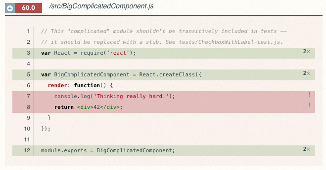 (Coverage of BigComplicatedComponent. Note that its
 (Debugging a React/Mocha test with node-inspector. Note that this is transpiled code.)
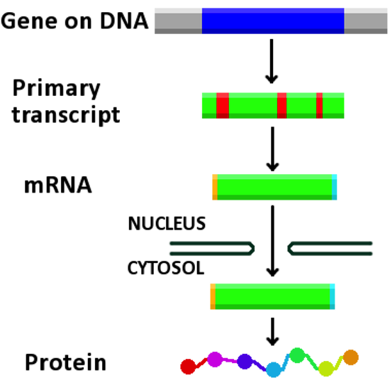